如果你也在 怎样代写凸优化Convex Optimization这个学科遇到相关的难题,请随时右上角联系我们的24/7代写客服。
凸优化是数学优化的一个子领域,研究的是凸集上凸函数最小化的问题。许多类凸优化问题都有多项时间算法,而数学优化一般来说是NP困难的。
statistics-lab™ 为您的留学生涯保驾护航 在代写凸优化Convex Optimization方面已经树立了自己的口碑, 保证靠谱, 高质且原创的统计Statistics代写服务。我们的专家在代写凸优化Convex Optimization代写方面经验极为丰富,各种代写凸优化Convex Optimization相关的作业也就用不着说。
我们提供的凸优化Convex Optimization及其相关学科的代写,服务范围广, 其中包括但不限于:
- Statistical Inference 统计推断
- Statistical Computing 统计计算
- Advanced Probability Theory 高等概率论
- Advanced Mathematical Statistics 高等数理统计学
- (Generalized) Linear Models 广义线性模型
- Statistical Machine Learning 统计机器学习
- Longitudinal Data Analysis 纵向数据分析
- Foundations of Data Science 数据科学基础
数学代写|凸优化作业代写Convex Optimization代考|Summary and discussion
In this chapter, we have revisited some mathematical basics of sets, functions, matrices, and vector spaces that will be very useful to understand the remaining chapters and we also introduced the notations that will be used throughout this book. The mathematical preliminaries reviewed in this chapter are by no means complete. For further details, the readers can refer to [Apo07] and [WZ97] for Section 1.1, and [H.J85] and [MS00] for Section 1.2, and other related textbooks.
Suppose that we are given an optimization problem in the following form:
$$
\begin{aligned}
\text { minimize } & f(\boldsymbol{x}) \
\text { subject to } & \boldsymbol{x} \in \mathcal{C}
\end{aligned}
$$
where $f(\boldsymbol{x})$ is the objective function to be minimized and $\mathcal{C}$ is the feasible set from which we try to find an optimal solution. Convex optimization itself is a powerful mathematical tool for optimally solving a well-defined convex optimization problem (i.e., $f(\boldsymbol{x})$ is a convex function and $\mathcal{C}$ is a convex set in problem $(1.127)$ ), or for handling a nonconvex optimization problem (that can be approximated as a convex one). However, the problem (1.127) under investigation may often appear to be a nonconvex optimization problem (with various camouflages) or a nonconvex and nondeterministic polynomial-time hard (NP-hard) problem that forces us to find an approximate solution with some performance or computational efficiency merits and characteristics instead. Furthermore, reformulation of the considered optimization problem into a convex optimization problem can be quite challenging. Fortunately, there are many problem reformulation approaches (e.g., function transformation, change of variables, and equivalent representations) to conversion of a nonconvex problem into a convex problem (i.e., unveiling of all the camouflages of the original problem).
The bridge between the pure mathematical convex optimization theory and how to use it in practical applications is the key for a successful researcher or professional who can efficiently exert his (her) efforts on solving a challenging scientific and engineering problem to which he (she) is dedicated. For a given opti-
mization problem, we aim to design an algorithm (e.g., transmit beamforming algorithm and resource allocation algorithm in communications and networking, nonnegative blind source separation algorithm for the analysis of biomedical and hyperspectral images) to efficiently and reliably yield a desired solution (that may just be an approximate solution rather than an optimal solution), as shown in Figure 1.6, where the block “Problem Reformulation,” the block “Algorithm Design,” and the block “Performance Evaluation and Analysis” are essential design steps before an algorithm that meets our goal is obtained. These design steps rely on smart use of advisable optimization theory and tools that remain in the cloud, like a military commander who needs not only ammunition and weapons but also an intelligent fighting strategy. It is quite helpful to build a bridge so that one can readily use any suitable mathematical theory (e.g., convex sets and functions, optimality conditions, duality, KKT conditions, Schur complement, S-procedure, etc.) and convex solvers (e.g., CVX and SeDuMi) to accomplish these design steps.
The ensuing chapters will introduce fundamental elements of the convex optimization theory in the cloud on one hand and illustrate how these elements were collectively applied in some successful cutting edge researches in communications and signal processing through the design procedure shown in Figure $1.6$ on the other hand, provided that the solid bridges between the cloud and all the design blocks have been constructed.
数学代写|凸优化作业代写Convex Optimization代考|Lines and line segments
In this chapter we introduce convex sets and their representations, properties, illustrative examples, convexity preserving operations, and geometry of convex sets which have proven very useful in signal processing applications such as hyperspectral and biomedical image analysis. Then we introduce proper cones (convex cones), dual norms and dual cones, generalized inequalities, and separating and supporting hyperplanes. All the materials on convex sets introduced in this chapter are essential to convex functions, convex problems, and duality to be introduced in the ensuing chapters. From this chapter on, for simplicity, we may use $\mathbf{x}$ to denote a vector in $\mathbb{R}^{n}$ and $x_{1}, \ldots, x_{n}$ for its components without explicitly mentioning $\mathbf{x} \in \mathbb{R}^{n}$.
Mathematically, a line $\mathcal{L}\left(\mathbf{x}{1}, \mathbf{x}{2}\right)$ passing through two points $\mathbf{x}{1}$ and $\mathbf{x}{2}$ in $\mathbb{R}^{n}$ is the set defined as
$$
\mathcal{L}\left(\mathbf{x}{1}, \mathbf{x}{2}\right)=\left{\theta \mathbf{x}{1}+(1-\theta) \mathbf{x}{2}, \theta \in \mathbb{R}\right}, \mathbf{x}{1}, \mathbf{x}{2} \in \mathbb{R}^{n}
$$
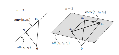
If $0 \leq \theta \leq 1$, then it is a line segment connecting $\mathbf{x}{1}$ and $\mathbf{x}{2}$. Note that the linear combination $\theta \mathbf{x}{1}+(1-\theta) \mathbf{x}{2}$ of two points $\mathbf{x}{1}$ and $\mathbf{x}{2}$ with the coefficient sum equal to unity as in (2.1) plays an essential role in defining affine sets and convex sets, and hence the one with $\theta \in \mathbb{R}$ is referred to as the affine combination and the one with $\theta \in[0,1]$ is referred to as the convex combination. Affine combination and convex combination can be extended to the case of more than two points in the same fashion.
Affine sets and affine hulls
A set $C$ is said to be an affine set if for any $\mathbf{x}{1}, \mathbf{x}{2} \in C$ and for any $\theta_{1}, \theta_{2} \in \mathbb{R}$ such that $\theta_{1}+\theta_{2}=1$, the point $\theta_{1} \mathbf{x}{1}+\theta{2} \mathbf{x}_{2}$ also belongs to the set $C$. For instance, the line defined in $(2.1)$ is an affine set. This concept can be extended to more than two points, as illustrated in the following example.
数学代写|凸优化作业代写Convex Optimization代考|Relative interior and relative boundary
Affine hull defined in (2.13) and affine dimension of a set defined in (2.14) play an essential role in convex geometric analysis, and have been applied to dimension reduction in many signal processing applications such as blind separation (or unmixing) of biomedical and hyperspectral image signals (to be introduced in Chapter 6). To further illustrate their characteristics, it would be useful to address the interior and the boundary of a set w.r.t. its affine hull, which are, respectively, termed as relative interior and relative boundary, and are defined below.
The relative interior of $C \subseteq \mathbb{R}^{n}$ is defined as
$$
\text { relint } \begin{aligned}
C &={\mathbf{x} \in C \mid B(\mathbf{x}, r) \cap \text { aff } C \subseteq C, \text { for some } r>0} \
&=\text { int } C \text { if aff } C=\mathbb{R}^{n} \quad(c f .(1.20)),
\end{aligned}
$$
where $B(\mathbf{x}, r)$ is a 2 -norm ball with center at $\mathbf{x}$ and radius $r$. It can be inferred from (2.16) that
$$
\text { int } C= \begin{cases}\text { relint } C, & \text { if affdim } C=n \ 0, & \text { otherwise. }\end{cases}
$$
The relative boundary of a set $C$ is defined as
$$
\begin{aligned}
\text { relbd } C &=\mathbf{c l} C \backslash \text { relint } C \
&=\mathbf{b d} C \text {, if int } C \neq \emptyset \text { (by }(2.17))
\end{aligned}
$$
For instance, for $C=\left{\mathbf{x} \in \mathbb{R}^{n} \mid|\mathbf{x}|_{\infty} \leq 1\right}$ (an infinity-norm ball), its interior and relative interior are identical, so are its boundary and relative boundary; for $C=\left{\mathbf{x}_{0}\right} \subset \mathbb{R}^{n}$ (a singleton set), int $C=\emptyset$ and bd $C=C$, but relbd $C=\emptyset$. Note that affdim $(C)=n$ for the former but affdim $(C)=0 \neq n$ for the latter, thereby providing the information of differentiating the interior (boundary) and the relative interior (relative boundary) of a set. Some more examples about the relative interior (relative boundary) of $C$ and the interior (boundary) of $C$, are illustrated in the following examples.
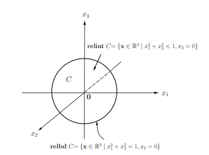
Example 2.2 Let $C=\left{\mathrm{x} \in \mathbb{R}^{3} \mid x_{1}^{2}+x_{3}^{2} \leq 1, x_{2}=0\right}=\mathrm{cl} C$. Then relint $C=$ $\left{\mathbf{x} \in \mathbb{R}^{3} \mid x_{1}^{2}+x_{3}^{2}<1, x_{2}=0\right}$ and relbd $C=\left{\mathbf{x} \in \mathbb{R}^{3} \mid x_{1}^{2}+x_{3}^{2}=1, x_{2}=0\right}$ as shown in Figure $2.3$. Note that int $C=\emptyset$ since affdim $(C)=2<3$, while bd $C=$ cl $C \backslash$ int $C=C$.
Example $2.3$ Let $C_{1}=\left{\mathbf{x} \in \mathbb{R}^{3} \mid|\mathbf{x}|_{2} \leq 1\right}$ and $C_{2}=\left{\mathbf{x} \in \mathbb{R}^{3} \mid|\mathbf{x}|_{2}=1\right}$. Then int $C_{1}=\left{\mathbf{x} \in \mathbb{R}^{3} \mid|\mathbf{x}|_{2}<1\right}=$ relint $C_{1}$ and int $C_{2}=$ relint $C_{2}=0$ due to $\operatorname{affdim}\left(C_{1}\right)=\operatorname{affdim}\left(C_{2}\right)=3$.
From now on, for the conceptual conciseness and clarity in the following introduction to convex sets, sometimes we address the pair (int $C$, bd $C$ ) in the context without explicitly mentioning that a convex set $C$ has nonempty interior. However, when int $C=\emptyset$ in the context, one can interpret the pair (int $C$, bd $C$ ) as the pair (relint $C$, relbd $C$ ).
凸优化代写
数学代写|凸优化作业代写Convex Optimization代考|Summary and discussion
在本章中,我们重温了集合、函数、矩阵和向量空间的一些数学基础知识,这对于理解其余章节非常有用,我们还介绍了将在本书中使用的符号。本章回顾的数学预备知识绝不是完整的。更详细的内容,读者可以参考[Apo07]和[WZ97]的1.1节,以及[H.J85]和[MS00]的1.2节,以及其他相关教材。
假设我们有一个如下形式的优化问题:
最小化 F(X) 受制于 X∈C
在哪里F(X)是要最小化的目标函数,并且C是我们试图从中找到最优解的可行集。凸优化本身是一个强大的数学工具,用于优化解决定义明确的凸优化问题(即,F(X)是一个凸函数并且C是问题中的凸集(1.127)),或用于处理非凸优化问题(可以近似为凸优化问题)。然而,正在研究的问题 (1.127) 可能经常看起来是一个非凸优化问题(有各种伪装)或一个非凸和非确定性多项式时间难 (NP-hard) 问题,它迫使我们找到具有某种性能或相反,计算效率的优点和特点。此外,将考虑的优化问题重新表述为凸优化问题可能非常具有挑战性。幸运的是,有许多问题重构方法(例如,函数变换、变量变化和等效表示)可以将非凸问题转换为凸问题(即揭示原始问题的所有伪装)。
纯数学凸优化理论与如何将其应用于实际应用之间的桥梁是成功的研究人员或专业人员能够有效地发挥他(她)的努力来解决他(她)所面临的具有挑战性的科学和工程问题的关键。投入的。对于给定的选项
化问题,我们的目标是设计一种算法(例如,通信和网络中的传输波束成形算法和资源分配算法,用于分析生物医学和高光谱图像的非负盲源分离算法)以有效且可靠地产生所需的解决方案(可能只是是近似解而不是最优解),如图 1.6 所示,其中“问题重构”模块、“算法设计”模块和“性能评估与分析”模块是算法满足之前的基本设计步骤我们的目标达到了。这些设计步骤依赖于明智地使用保留在云中的可取优化理论和工具,例如军事指挥官,他不仅需要弹药和武器,还需要智能战斗策略。
随后的章节将一方面介绍云中凸优化理论的基本要素,并说明这些要素如何通过图 1 所示的设计过程共同应用于通信和信号处理领域的一些成功的前沿研究中。1.6另一方面,前提是云和所有设计块之间的坚固桥梁已经构建。
数学代写|凸优化作业代写Convex Optimization代考|Lines and line segments
在本章中,我们将介绍凸集及其表示、属性、说明性示例、凸性保持操作以及凸集的几何形状,这些在高光谱和生物医学图像分析等信号处理应用中已被证明非常有用。然后我们介绍了真锥(凸锥)、对偶范数和对偶锥、广义不等式以及分离和支持超平面。本章介绍的所有关于凸集的材料对于后续章节中介绍的凸函数、凸问题和对偶都是必不可少的。从本章开始,为简单起见,我们可以使用X表示一个向量Rn和X1,…,Xn对于它的组件,没有明确提及X∈Rn.
在数学上,一条线大号(X1,X2)通过两点X1和X2在Rn是定义为的集合
\mathcal{L}\left(\mathbf{x}{1}, \mathbf{x}{2}\right)=\left{\theta \mathbf{x}{1}+(1-\theta) \ mathbf{x}{2}, \theta \in \mathbb{R}\right}, \mathbf{x}{1}, \mathbf{x}{2} \in \mathbb{R}^{n}\mathcal{L}\left(\mathbf{x}{1}, \mathbf{x}{2}\right)=\left{\theta \mathbf{x}{1}+(1-\theta) \ mathbf{x}{2}, \theta \in \mathbb{R}\right}, \mathbf{x}{1}, \mathbf{x}{2} \in \mathbb{R}^{n}
如果0≤θ≤1,那么它就是一条连接线段X1和X2. 注意线性组合θX1+(1−θ)X2两点X1和X2系数和等于(2.1)中的单位在定义仿射集和凸集方面起着重要作用,因此具有θ∈R被称为仿射组合和一个与θ∈[0,1]称为凸组合。仿射组合和凸组合可以以相同的方式扩展到两个以上点的情况。
仿射集和仿射壳
A 集C被称为仿射集,如果对于任何X1,X2∈C并且对于任何θ1,θ2∈R这样θ1+θ2=1, 点θ1X1+θ2X2也属于集合C. 例如,定义在(2.1)是一个仿射集。这个概念可以扩展到两点以上,如下例所示。
数学代写|凸优化作业代写Convex Optimization代考|Relative interior and relative boundary
(2.13)中定义的仿射壳和(2.14)中定义的集合的仿射维数在凸几何分析中发挥着重要作用,并已应用于许多信号处理应用中的降维,例如生物医学和高光谱图像信号(将在第 6 章中介绍)。为了进一步说明它们的特性,有必要通过其仿射壳来解决集合的内部和边界,它们分别称为相对内部和相对边界,并在下面定义。
相对内部C⊆Rn定义为
重新安装 C=X∈C∣乙(X,r)∩ 亲 C⊆C, 对于一些 r>0 = 整数 C 如果 C=Rn(CF.(1.20)),
在哪里乙(X,r)是一个 2 范数球,中心在X和半径r. 由式(2.16)可以推导出
整数 C={ 重新安装 C, 如果 affdim C=n 0, 除此以外。
集合的相对边界C定义为
重磅 C=ClC∖ 重新安装 C =bdC, 如果 int C≠∅ (经过 (2.17))
例如,对于C=\left{\mathbf{x} \in \mathbb{R}^{n} \mid|\mathbf{x}|_{\infty} \leq 1\right}C=\left{\mathbf{x} \in \mathbb{R}^{n} \mid|\mathbf{x}|_{\infty} \leq 1\right}(一个无穷范数球),它的内部和相对内部是相同的,它的边界和相对边界也是相同的;为了C=\left{\mathbf{x}_{0}\right} \subset \mathbb{R}^{n}C=\left{\mathbf{x}_{0}\right} \subset \mathbb{R}^{n}(单例集),intC=∅和 bdC=C, 但是 relbdC=∅. 注意 affdim(C)=n对于前者但 affdim(C)=0≠n对于后者,从而提供区分集合的内部(边界)和相对内部(相对边界)的信息。关于相对内部(相对边界)的更多示例C和内部(边界)C,在以下示例中进行了说明。
例 2.2 让C=\left{\mathrm{x} \in \mathbb{R}^{3} \mid x_{1}^{2}+x_{3}^{2} \leq 1, x_{2}=0 \right}=\mathrm{cl} CC=\left{\mathrm{x} \in \mathbb{R}^{3} \mid x_{1}^{2}+x_{3}^{2} \leq 1, x_{2}=0 \right}=\mathrm{cl} C. 然后重振旗鼓C= \left{\mathbf{x} \in \mathbb{R}^{3} \mid x_{1}^{2}+x_{3}^{2}<1, x_{2}=0\right}\left{\mathbf{x} \in \mathbb{R}^{3} \mid x_{1}^{2}+x_{3}^{2}<1, x_{2}=0\right}和 relbdC=\left{\mathbf{x} \in \mathbb{R}^{3} \mid x_{1}^{2}+x_{3}^{2}=1, x_{2}=0\对}C=\left{\mathbf{x} \in \mathbb{R}^{3} \mid x_{1}^{2}+x_{3}^{2}=1, x_{2}=0\对}如图2.3. 请注意,intC=∅自从 affdim(C)=2<3, 而 bdC=分类C∖整数C=C.
例子2.3让C_{1}=\left{\mathbf{x} \in \mathbb{R}^{3} \mid|\mathbf{x}|_{2} \leq 1\right}C_{1}=\left{\mathbf{x} \in \mathbb{R}^{3} \mid|\mathbf{x}|_{2} \leq 1\right}和C_{2}=\left{\mathbf{x} \in \mathbb{R}^{3} \mid|\mathbf{x}|_{2}=1\right}C_{2}=\left{\mathbf{x} \in \mathbb{R}^{3} \mid|\mathbf{x}|_{2}=1\right}. 然后 intC_{1}=\left{\mathbf{x} \in \mathbb{R}^{3} \mid|\mathbf{x}|_{2}<1\right}=C_{1}=\left{\mathbf{x} \in \mathbb{R}^{3} \mid|\mathbf{x}|_{2}<1\right}=重新安装C1和整数C2=重新安装C2=0由于关注(C1)=关注(C2)=3.
从现在开始,为了在下面对凸集的介绍中概念简洁明了,有时我们会讨论对(intC, bdC) 在上下文中没有明确提到凸集C有非空的内部。但是,当 intC=∅在上下文中,人们可以解释这对(intC, bdC) 作为对 (relintC, relbdC ).

统计代写请认准statistics-lab™. statistics-lab™为您的留学生涯保驾护航。
金融工程代写
金融工程是使用数学技术来解决金融问题。金融工程使用计算机科学、统计学、经济学和应用数学领域的工具和知识来解决当前的金融问题,以及设计新的和创新的金融产品。
非参数统计代写
非参数统计指的是一种统计方法,其中不假设数据来自于由少数参数决定的规定模型;这种模型的例子包括正态分布模型和线性回归模型。
广义线性模型代考
广义线性模型(GLM)归属统计学领域,是一种应用灵活的线性回归模型。该模型允许因变量的偏差分布有除了正态分布之外的其它分布。
术语 广义线性模型(GLM)通常是指给定连续和/或分类预测因素的连续响应变量的常规线性回归模型。它包括多元线性回归,以及方差分析和方差分析(仅含固定效应)。
有限元方法代写
有限元方法(FEM)是一种流行的方法,用于数值解决工程和数学建模中出现的微分方程。典型的问题领域包括结构分析、传热、流体流动、质量运输和电磁势等传统领域。
有限元是一种通用的数值方法,用于解决两个或三个空间变量的偏微分方程(即一些边界值问题)。为了解决一个问题,有限元将一个大系统细分为更小、更简单的部分,称为有限元。这是通过在空间维度上的特定空间离散化来实现的,它是通过构建对象的网格来实现的:用于求解的数值域,它有有限数量的点。边界值问题的有限元方法表述最终导致一个代数方程组。该方法在域上对未知函数进行逼近。[1] 然后将模拟这些有限元的简单方程组合成一个更大的方程系统,以模拟整个问题。然后,有限元通过变化微积分使相关的误差函数最小化来逼近一个解决方案。
tatistics-lab作为专业的留学生服务机构,多年来已为美国、英国、加拿大、澳洲等留学热门地的学生提供专业的学术服务,包括但不限于Essay代写,Assignment代写,Dissertation代写,Report代写,小组作业代写,Proposal代写,Paper代写,Presentation代写,计算机作业代写,论文修改和润色,网课代做,exam代考等等。写作范围涵盖高中,本科,研究生等海外留学全阶段,辐射金融,经济学,会计学,审计学,管理学等全球99%专业科目。写作团队既有专业英语母语作者,也有海外名校硕博留学生,每位写作老师都拥有过硬的语言能力,专业的学科背景和学术写作经验。我们承诺100%原创,100%专业,100%准时,100%满意。
随机分析代写
随机微积分是数学的一个分支,对随机过程进行操作。它允许为随机过程的积分定义一个关于随机过程的一致的积分理论。这个领域是由日本数学家伊藤清在第二次世界大战期间创建并开始的。
时间序列分析代写
随机过程,是依赖于参数的一组随机变量的全体,参数通常是时间。 随机变量是随机现象的数量表现,其时间序列是一组按照时间发生先后顺序进行排列的数据点序列。通常一组时间序列的时间间隔为一恒定值(如1秒,5分钟,12小时,7天,1年),因此时间序列可以作为离散时间数据进行分析处理。研究时间序列数据的意义在于现实中,往往需要研究某个事物其随时间发展变化的规律。这就需要通过研究该事物过去发展的历史记录,以得到其自身发展的规律。
回归分析代写
多元回归分析渐进(Multiple Regression Analysis Asymptotics)属于计量经济学领域,主要是一种数学上的统计分析方法,可以分析复杂情况下各影响因素的数学关系,在自然科学、社会和经济学等多个领域内应用广泛。
MATLAB代写
MATLAB 是一种用于技术计算的高性能语言。它将计算、可视化和编程集成在一个易于使用的环境中,其中问题和解决方案以熟悉的数学符号表示。典型用途包括:数学和计算算法开发建模、仿真和原型制作数据分析、探索和可视化科学和工程图形应用程序开发,包括图形用户界面构建MATLAB 是一个交互式系统,其基本数据元素是一个不需要维度的数组。这使您可以解决许多技术计算问题,尤其是那些具有矩阵和向量公式的问题,而只需用 C 或 Fortran 等标量非交互式语言编写程序所需的时间的一小部分。MATLAB 名称代表矩阵实验室。MATLAB 最初的编写目的是提供对由 LINPACK 和 EISPACK 项目开发的矩阵软件的轻松访问,这两个项目共同代表了矩阵计算软件的最新技术。MATLAB 经过多年的发展,得到了许多用户的投入。在大学环境中,它是数学、工程和科学入门和高级课程的标准教学工具。在工业领域,MATLAB 是高效研究、开发和分析的首选工具。MATLAB 具有一系列称为工具箱的特定于应用程序的解决方案。对于大多数 MATLAB 用户来说非常重要,工具箱允许您学习和应用专业技术。工具箱是 MATLAB 函数(M 文件)的综合集合,可扩展 MATLAB 环境以解决特定类别的问题。可用工具箱的领域包括信号处理、控制系统、神经网络、模糊逻辑、小波、仿真等。