如果你也在 怎样代写复变函数Complex function这个学科遇到相关的难题,请随时右上角联系我们的24/7代写客服。
复数函数是一个从复数到复数的函数。换句话说,它是一个以复数的一个子集为域,以复数为子域的函数。复数函数通常应该有一个包含复数平面的非空开放子集的域。
statistics-lab™ 为您的留学生涯保驾护航 在代写复变函数Complex function方面已经树立了自己的口碑, 保证靠谱, 高质且原创的统计Statistics代写服务。我们的专家在代写复变函数Complex function代写方面经验极为丰富,各种代写复变函数Complex function相关的作业也就用不着说。
我们提供的复变函数Complex function及其相关学科的代写,服务范围广, 其中包括但不限于:
- Statistical Inference 统计推断
- Statistical Computing 统计计算
- Advanced Probability Theory 高等概率论
- Advanced Mathematical Statistics 高等数理统计学
- (Generalized) Linear Models 广义线性模型
- Statistical Machine Learning 统计机器学习
- Longitudinal Data Analysis 纵向数据分析
- Foundations of Data Science 数据科学基础
数学代写|复变函数作业代写Complex function代考|The Cauchy Estimates and Liouville’s Theorem
This section will establish some estimates for the derivatives of holomorphic functions in terms of bounds on the function itself. The possibility
of such estimation is a feature of holomorphic function theory that has no analogue in the theory of real variables. For example: The functions $f_{k}(x)=\sin k x, x \in \mathbb{R}, k \in \mathbb{Z}$, are for all $k$ bounded in absolute value by 1 ; but their derivatives at 0 are not bounded since $f_{k}^{\prime}(0)=k$. The reader should think frequently about the ways in which real function theory and complex holomorphic function theory differ. In the subject matter of this section, the differences are particularly pronounced.
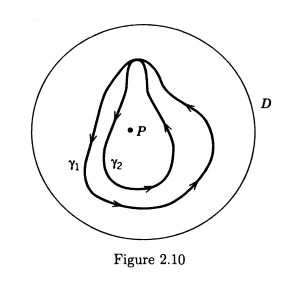
Theorem 3.4.1 (The Cauchy estimates). Let $f: U \rightarrow \mathbb{C}$ be a holomorphic function on an open set $U, P \in U$, and assume that the closed disc $\bar{D}(P, r), r>0$, is contained in $U$. Set $M=\sup {z \in \bar{D}(P, r)}|f(z)|$. Then for $k=1,2,3 \ldots$ we have $$ \left|\frac{\partial^{k} f}{\partial z^{k}}(P)\right| \leq \frac{M k !}{r^{k}} $$ Proof. By Theorem 3.1.1, $$ \frac{\partial^{k} f}{\partial z^{k}}(P)=\frac{k !}{2 \pi i} \oint{|\zeta-P|=r} \frac{f(\zeta)}{(\zeta-P)^{k+1}} d \zeta
$$
Now we use Proposition 2.1.8 to see that
$$
\left|\frac{\partial^{k} f}{\partial z^{k}}(P)\right| \leq \frac{k !}{2 \pi} \cdot 2 \pi r \sup {|\zeta-P|=r} \frac{|f|}{|\zeta-P|^{k+1}} \leq \frac{M k !}{r^{k}} $$ Notice that the Cauchy estimates enable one to estimate directly the radius of convergence of the power series $$ \sum \frac{f^{(k)}(P)}{k !}(z-P)^{k} $$ Namely $$ \limsup {k \rightarrow+\infty}\left|\frac{f^{(k)}(P)}{k !}\right|^{1 / k} \leq \limsup {k \rightarrow+\infty}\left|\frac{M \cdot k !}{r^{k}} \cdot \frac{1}{k !}\right|^{1 / k}=\frac{1}{r} $$ for any $r$ such that $\bar{D}(P, r) \subseteq U$. In particular, the radius of convergence, which equals $$ \left[\limsup {k \rightarrow+\infty}\left|\frac{f^{(k)}(P)}{k !}\right|^{1 / k}\right]^{-1}
$$
is at least $1 /(1 / r)=r$ for all $r$ such that $\bar{D}(P, r) \subseteq U$. Hence the radius of convergence is at least as large as the distance from $P$ to $\mathbb{C} \backslash U$ (this result was considered from a different perspective in Theorem 3.3.1).
The derivative bounds of Theorem 3.4.1 have some remarkable consequences. The first one is the fact that a holomorphic function on $\mathbb{C}$ that is bounded in absolute value is in fact constant. We shall need the following lemma to prove this.
数学代写|复变函数作业代写Complex function代考|Uniform Limits of Holomorphic Functions
We have already seen that a convergent power series (in $z$ ) defines a holomorphic function (Lemma 3.2.10). One can think of this fact as the assertion that a certain sequence of holomorphic functions, namely the finite partial sums of the series, has a holomorphic limit. This idea, that a limit of holomorphic functions is holomorphic, holds in almost unrestricted generality.
Theorem 3.5.1. Let $f_{j}: U \rightarrow \mathbb{C}, j=1,2,3 \ldots$, be a sequence of holomorphic functions on an open set $U$ in $\mathbb{C}$. Suppose that there is a function $f: U \rightarrow \mathbb{C}$ such that, for each compact subset $E$ of $U$, the sequence $\left.f_{j}\right|{E}$ converges uniformly to $\left.f\right|{E}$. Then $f$ is holomorphic on $U$. (In particular, $\left.f \in C^{\infty}(U)_{.}\right)$
Before beginning the proof, we again note the contrast with the realvariable situation. Any continuous function from $\mathbb{R}$ to $\mathbb{R}$ is the limit, uniformly on compact subsets of $\mathbb{R}$, of some sequence of polynomials: This is the well-known Weierstrass approximation theorem. But, of course, a continuous function from $\mathbb{R}$ to $\mathbb{R}$ certainly need not be real analytic, or even $C^{\infty}$. The difference between the real-variable situation and that of the theorem is related to the Cauchy estimates. The convergence of a sequence of holomorphic functions implies convergence of their derivatives also. No such estimation holds in the real case, and a sequence of $C^{\infty}$ functions can converge uniformly without their derivatives having any convergence properties at all (see Exercise 1 and [RUD1]).
We shall give one detailed proof of Theorem 3.5.1 and sketch a second. The first method is especially brief.
Proof of Theorem 3.5.1. Let $P \in U$ be arbitrary. Then choose $r>0$ such that $\bar{D}(P, r) \subseteq U$. Since $\left{f_{j}\right}$ converges to $f$ uniformly on $\bar{D}(P, r)$ and since each $f_{j}$ is continuous, $f$ is also continuous on $\bar{D}(P, r)$. For any $z \in D(P, r)$
数学代写|复变函数作业代写Complex function代考|The Zeros of a Holomorphic Function
Let $f$ be a holomorphic function. If $f$ is not identically zero, then it turns out that $f$ cannot vanish at too many points. This once again bears out the dictum that holomorphic functions are a lot like polynomials. The idea has a precise formulation as follows:
Theorem 3.6.1. Let $U \subseteq \mathbb{C}$ be a connected open set and let $f: U \rightarrow \mathbb{C}$ be holomorphic. Let $\mathbf{Z}={z \in U: f(z)=0}$. If there are a $z_{0} \in \mathbf{Z}$ and $\left{z_{j}\right}_{j=1}^{\infty} \subseteq \mathbf{Z} \backslash\left{z_{0}\right}$ such that $z_{j} \rightarrow z_{0}$, then $f \equiv 0$.
Let us formulate Theorem $3.6 .1$ in topological terms. We recall that a point $z_{0}$ is said to be an accumulation point of a set $Z$ if there is a sequence $\left{z_{j}\right} \subseteq Z \backslash\left{z_{0}\right}$ with $\lim {j \rightarrow \infty} z{j}=z_{0}$. Then Theorem $3.6 .1$ is equivalent to the statement: If $f: U \rightarrow \mathbb{C}$ is a holomorphic function on a connected open set $U$ and if $Z={z \in U: f(z)=0}$ has an accumulation point in $U$, then $f \equiv 0$.
There is still more terminology attached to the situation in Theorem 3.6.1. A set $S$ is said to be discrete if for each $s \in S$ there is an $\epsilon>0$ such that $D(s, \epsilon) \cap S={s}$. People also say, in an abuse of language, that a discrete set has points which are “isolated” or that $S$ contains only “isolated points.” Theorem 3.6.1 thus asserts that if $f$ is a nonconstant holomorphic function on a connected open set, then its zero set is discrete or, less formally, the zeros of $f$ are isolated. It is important to realize that Theorem 3.6.1 does not rule out the possibility that the zero set of $f$ can have accumulation points in $\mathbb{C} \backslash U$; in particular, a nonconstant holomorphic function on an open set $U$ can indeed have zeros accumulating at a point of $\partial U$. For example, the function $f(z)=\sin (1 /(1-z))$ is holomorphic on $U=D(0,1)$ and vanishes on the set
$$
\mathbf{Z}=\left{1-\frac{1}{\pi n}: n=1,2,3, \ldots\right} .
$$
Plainly $\mathbf{Z}$ has no accumulation points in $U$; however the point $1 \in \partial U$ is an accumulation point of $\mathbf{Z}$.
Proof of Theorem 3.6.1. We first claim that, under the hypotheses of the theorem, $(\partial / \partial z)^{n} f\left(z_{0}\right)=0$ for every nonnegative integer $n$. If this is not the case, let $n_{0}$ be the least nonnegative integer $n$ such that
$$
\left(\frac{\partial}{\partial z}\right)^{n_{0}} f\left(z_{0}\right) \neq 0
$$
Then we have, on some small disc $D\left(z_{0}, r\right)$, the power series expansion
$$
f(z)=\sum_{j=n_{0}}^{\infty}\left(\frac{\partial^{j}}{\partial z^{j}} f\left(z_{0}\right)\right) \frac{\left(z-z_{0}\right)^{j}}{j !} .
$$
Therefore the function $g$ defined by
$$
g(z) \equiv \sum_{j=n_{0}}^{\infty}\left(\frac{\partial}{\partial z}\right)^{j} f\left(z_{0}\right) \frac{\left(z-z_{0}\right)^{j-n_{0}}}{j !}
$$
is holomorphic on $D\left(z_{0}, r\right)$ and $g\left(z_{0}\right) \neq 0$ since $\left(\frac{\partial}{\partial z}\right)^{n_{0}} f\left(z_{0}\right) \neq 0$. Notice that the indicated power series has the same radius of convergence as that for $f$ itself. Furthermore, $g\left(z_{l}\right)=0$ for $l=1,2,3, \ldots$. But then, by the continuity of $g, g\left(z_{0}\right)=0$. This contradiction proves our claim.
复变函数代写
数学代写|复变函数作业代写Complex function代考|The Cauchy Estimates and Liouville’s Theorem
本节将根据函数本身的界限对全纯函数的导数建立一些估计。可能性
这种估计是全纯函数理论的一个特点,在实变量理论中没有类似物。例如:函数Fķ(X)=罪ķX,X∈R,ķ∈从, 适用于所有人ķ绝对值以 1 为界;但它们在 0 处的导数是无界的,因为Fķ′(0)=ķ. 读者应该经常思考实函数论和复全纯函数论的不同之处。在本节的主题中,差异尤其明显。
定理 3.4.1(柯西估计)。让F:在→C是开集上的全纯函数在,磷∈在, 并假设闭合圆盘D¯(磷,r),r>0, 包含在在. 放米=支持和∈D¯(磷,r)|F(和)|. 那么对于ķ=1,2,3…我们有|∂ķF∂和ķ(磷)|≤米ķ!rķ证明。根据定理 3.1.1,∂ķF∂和ķ(磷)=ķ!2圆周率一世∮|G−磷|=rF(G)(G−磷)ķ+1dG
现在我们使用命题 2.1.8 来看看
|∂ķF∂和ķ(磷)|≤ķ!2圆周率⋅2圆周率r支持|G−磷|=r|F||G−磷|ķ+1≤米ķ!rķ请注意,柯西估计使人们能够直接估计幂级数的收敛半径∑F(ķ)(磷)ķ!(和−磷)ķ即林汤ķ→+∞|F(ķ)(磷)ķ!|1/ķ≤林汤ķ→+∞|米⋅ķ!rķ⋅1ķ!|1/ķ=1r对于任何r这样D¯(磷,r)⊆在. 特别是,收敛半径等于[林汤ķ→+∞|F(ķ)(磷)ķ!|1/ķ]−1
至少是1/(1/r)=r对全部r这样D¯(磷,r)⊆在. 因此,收敛半径至少与距离的距离一样大磷到C∖在(这个结果在定理 3.3.1 中从不同的角度考虑)。
定理 3.4.1 的导数界限有一些显着的结果。第一个是一个全纯函数C有界的绝对值实际上是常数。我们需要以下引理来证明这一点。
数学代写|复变函数作业代写Complex function代考|Uniform Limits of Holomorphic Functions
We have already seen that a convergent power series (in z ) defines a holomorphic function (Lemma 3.2.10). One can think of this fact as the assertion that a certain sequence of holomorphic functions, namely the finite partial sums of the series, has a holomorphic limit. This idea, that a limit of holomorphic functions is holomorphic, holds in almost unrestricted generality.
Theorem 3.5.1. Let fj:U→C,j=1,2,3…, be a sequence of holomorphic functions on an open set U in C. Suppose that there is a function f:U→C such that, for each compact subset E of U, the sequence fj|E converges uniformly to f|E. Then f is holomorphic on U. (In particular, f∈C∞(U).)
Before beginning the proof, we again note the contrast with the realvariable situation. Any continuous function from R to R是限制,一致地在紧凑子集上R, 一些多项式序列:这是著名的 Weierstrass 逼近定理。但是,当然,一个连续的函数R到R当然不必是真正的分析,甚至C∞. 实变量情况与定理的区别与柯西估计有关。一系列全纯函数的收敛也意味着它们的导数的收敛。在实际情况中没有这样的估计,并且一系列C∞函数可以均匀收敛,而它们的导数根本不具有任何收敛特性(参见练习 1 和 [RUD1])。
我们将给出定理 3.5.1 的一个详细证明,并画出第二个。第一种方法特别简短。
定理 3.5.1 的证明。让磷∈在随意。然后选择r>0这样D¯(磷,r)⊆在. 自从\左{f_{j}\右}\左{f_{j}\右}收敛到F一致地D¯(磷,r)并且由于每个Fj是连续的,F也是连续的D¯(磷,r). 对于任何和∈D(磷,r)
数学代写|复变函数作业代写Complex function代考|The Zeros of a Holomorphic Function
让F是一个全纯函数。如果F不完全为零,那么事实证明F不能在太多点消失。这再次证实了全纯函数很像多项式的格言。这个想法有一个精确的表述如下:
定理 3.6.1。让在⊆C是一个连通的开集并且让F:在→C是全纯的。让从=和∈在:F(和)=0. 如果有一个和0∈从和\left{z_{j}\right}_{j=1}^{\infty} \subseteq \mathbf{Z} \backslash\left{z_{0}\right}\left{z_{j}\right}_{j=1}^{\infty} \subseteq \mathbf{Z} \backslash\left{z_{0}\right}这样和j→和0, 然后F≡0.
让我们制定定理3.6.1在拓扑方面。我们记得有一点和0据说是一个集合的一个累积点从如果有序列\left{z_{j}\right} \subseteq Z \backslash\left{z_{0}\right}\left{z_{j}\right} \subseteq Z \backslash\left{z_{0}\right}与 $\lim {j \rightarrow \infty} z {j}=z_{0}.吨H和n吨H和这r和米3.6 .1一世s和q在一世在一种l和n吨吨这吨H和s吨一种吨和米和n吨:一世Ff: U \rightarrow \mathbb{C}一世s一种H这l这米这rpH一世CF在nC吨一世这n这n一种C这nn和C吨和d这p和ns和吨在一种nd一世FZ={z \in U: f(z)=0}H一种s一种n一种CC在米在l一种吨一世这np这一世n吨一世n在,吨H和nf \equiv 0$。
定理 3.6.1 中的情况还有更多的术语。一套小号被称为是离散的,如果对于每个s∈小号有一个ε>0这样D(s,ε)∩小号=s. 人们还说,在滥用语言的情况下,离散集合具有“孤立”的点,或者小号仅包含“孤立点”。因此,定理 3.6.1 断言如果F是连通开集上的非常量全纯函数,则其零集是离散的,或者更正式地说,零集F被隔离。重要的是要认识到定理 3.6.1 不排除零集的可能性F可以有积累点C∖在; 特别是开集上的非常数全纯函数在确实可以在某个点累积零∂在. 例如,函数F(和)=罪(1/(1−和))是全纯的在=D(0,1)然后消失在片场
\mathbf{Z}=\left{1-\frac{1}{\pi n}: n=1,2,3, \ldots\right} 。\mathbf{Z}=\left{1-\frac{1}{\pi n}: n=1,2,3, \ldots\right} 。
说白了从没有累积积分在; 然而重点1∈∂在是一个积累点从.
定理 3.6.1 的证明。我们首先声称,在定理的假设下,(∂/∂和)nF(和0)=0对于每个非负整数n. 如果不是这种情况,让n0是最小的非负整数n这样
(∂∂和)n0F(和0)≠0
然后我们有,在一些小光盘上D(和0,r), 幂级数展开
F(和)=∑j=n0∞(∂j∂和jF(和0))(和−和0)jj!.
因此函数G被定义为
G(和)≡∑j=n0∞(∂∂和)jF(和0)(和−和0)j−n0j!
是全纯的D(和0,r)和G(和0)≠0自从(∂∂和)n0F(和0)≠0. 请注意,指示的幂级数具有与F本身。此外,G(和l)=0为了l=1,2,3,…. 但是,由于连续性G,G(和0)=0. 这个矛盾证明了我们的主张。

统计代写请认准statistics-lab™. statistics-lab™为您的留学生涯保驾护航。
金融工程代写
金融工程是使用数学技术来解决金融问题。金融工程使用计算机科学、统计学、经济学和应用数学领域的工具和知识来解决当前的金融问题,以及设计新的和创新的金融产品。
非参数统计代写
非参数统计指的是一种统计方法,其中不假设数据来自于由少数参数决定的规定模型;这种模型的例子包括正态分布模型和线性回归模型。
广义线性模型代考
广义线性模型(GLM)归属统计学领域,是一种应用灵活的线性回归模型。该模型允许因变量的偏差分布有除了正态分布之外的其它分布。
术语 广义线性模型(GLM)通常是指给定连续和/或分类预测因素的连续响应变量的常规线性回归模型。它包括多元线性回归,以及方差分析和方差分析(仅含固定效应)。
有限元方法代写
有限元方法(FEM)是一种流行的方法,用于数值解决工程和数学建模中出现的微分方程。典型的问题领域包括结构分析、传热、流体流动、质量运输和电磁势等传统领域。
有限元是一种通用的数值方法,用于解决两个或三个空间变量的偏微分方程(即一些边界值问题)。为了解决一个问题,有限元将一个大系统细分为更小、更简单的部分,称为有限元。这是通过在空间维度上的特定空间离散化来实现的,它是通过构建对象的网格来实现的:用于求解的数值域,它有有限数量的点。边界值问题的有限元方法表述最终导致一个代数方程组。该方法在域上对未知函数进行逼近。[1] 然后将模拟这些有限元的简单方程组合成一个更大的方程系统,以模拟整个问题。然后,有限元通过变化微积分使相关的误差函数最小化来逼近一个解决方案。
tatistics-lab作为专业的留学生服务机构,多年来已为美国、英国、加拿大、澳洲等留学热门地的学生提供专业的学术服务,包括但不限于Essay代写,Assignment代写,Dissertation代写,Report代写,小组作业代写,Proposal代写,Paper代写,Presentation代写,计算机作业代写,论文修改和润色,网课代做,exam代考等等。写作范围涵盖高中,本科,研究生等海外留学全阶段,辐射金融,经济学,会计学,审计学,管理学等全球99%专业科目。写作团队既有专业英语母语作者,也有海外名校硕博留学生,每位写作老师都拥有过硬的语言能力,专业的学科背景和学术写作经验。我们承诺100%原创,100%专业,100%准时,100%满意。
随机分析代写
随机微积分是数学的一个分支,对随机过程进行操作。它允许为随机过程的积分定义一个关于随机过程的一致的积分理论。这个领域是由日本数学家伊藤清在第二次世界大战期间创建并开始的。
时间序列分析代写
随机过程,是依赖于参数的一组随机变量的全体,参数通常是时间。 随机变量是随机现象的数量表现,其时间序列是一组按照时间发生先后顺序进行排列的数据点序列。通常一组时间序列的时间间隔为一恒定值(如1秒,5分钟,12小时,7天,1年),因此时间序列可以作为离散时间数据进行分析处理。研究时间序列数据的意义在于现实中,往往需要研究某个事物其随时间发展变化的规律。这就需要通过研究该事物过去发展的历史记录,以得到其自身发展的规律。
回归分析代写
多元回归分析渐进(Multiple Regression Analysis Asymptotics)属于计量经济学领域,主要是一种数学上的统计分析方法,可以分析复杂情况下各影响因素的数学关系,在自然科学、社会和经济学等多个领域内应用广泛。
MATLAB代写
MATLAB 是一种用于技术计算的高性能语言。它将计算、可视化和编程集成在一个易于使用的环境中,其中问题和解决方案以熟悉的数学符号表示。典型用途包括:数学和计算算法开发建模、仿真和原型制作数据分析、探索和可视化科学和工程图形应用程序开发,包括图形用户界面构建MATLAB 是一个交互式系统,其基本数据元素是一个不需要维度的数组。这使您可以解决许多技术计算问题,尤其是那些具有矩阵和向量公式的问题,而只需用 C 或 Fortran 等标量非交互式语言编写程序所需的时间的一小部分。MATLAB 名称代表矩阵实验室。MATLAB 最初的编写目的是提供对由 LINPACK 和 EISPACK 项目开发的矩阵软件的轻松访问,这两个项目共同代表了矩阵计算软件的最新技术。MATLAB 经过多年的发展,得到了许多用户的投入。在大学环境中,它是数学、工程和科学入门和高级课程的标准教学工具。在工业领域,MATLAB 是高效研究、开发和分析的首选工具。MATLAB 具有一系列称为工具箱的特定于应用程序的解决方案。对于大多数 MATLAB 用户来说非常重要,工具箱允许您学习和应用专业技术。工具箱是 MATLAB 函数(M 文件)的综合集合,可扩展 MATLAB 环境以解决特定类别的问题。可用工具箱的领域包括信号处理、控制系统、神经网络、模糊逻辑、小波、仿真等。