如果你也在 怎样代写复变函数Complex function这个学科遇到相关的难题,请随时右上角联系我们的24/7代写客服。
复数函数是一个从复数到复数的函数。换句话说,它是一个以复数的一个子集为域,以复数为子域的函数。复数函数通常应该有一个包含复数平面的非空开放子集的域。
statistics-lab™ 为您的留学生涯保驾护航 在代写复变函数Complex function方面已经树立了自己的口碑, 保证靠谱, 高质且原创的统计Statistics代写服务。我们的专家在代写复变函数Complex function代写方面经验极为丰富,各种代写复变函数Complex function相关的作业也就用不着说。
我们提供的复变函数Complex function及其相关学科的代写,服务范围广, 其中包括但不限于:
- Statistical Inference 统计推断
- Statistical Computing 统计计算
- Advanced Probability Theory 高等概率论
- Advanced Mathematical Statistics 高等数理统计学
- (Generalized) Linear Models 广义线性模型
- Statistical Machine Learning 统计机器学习
- Longitudinal Data Analysis 纵向数据分析
- Foundations of Data Science 数据科学基础
数学代写|复变函数作业代写Complex function代考|Cauchy Integral Theorem
In this section we shall study two results which are fundamental to the development of the rest of this subject: the Cauchy Integral Formula and the Cauchy integral theorem. The Cauchy integral formula gives the value of a holomorphic function at each point inside a circle in terms of the values of the function on the circle (later we shall learn that “circle” here may be replaced by a more general closed curve, subject to certain topological restrictions). We proceed now with our study of the Cauchy integral formula.
The Cauchy integral formula is so startling that one may at first be puzzled by it and find it unmotivated. However, as the theory develops, one can look at it in retrospect and see how natural it is. In any case it makes
possible the extremely rapid development of a very powerful theory, and a certain patience with the abruptness of its proof will be richly rewarded.
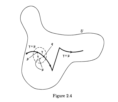
It will be useful to have at our disposal the following notation: If $P$ is a complex number, and $r$ a positive real number, then we let $D(P, r)={z \in$ $\mathbb{C}:|z-P|<r}$ and $\bar{D}(P, r)={z \in \mathbb{C}:|z-P| \leq r}$. These sets are called, respectively, open and closed discs in the complex plane. The boundary of the disc, $\partial D(P, r)$, is the set of $z$ such that $|z-P|=r$.
The boundary $\partial D(P, r)$ of the disc $D(P, r)$ can be parametrized as a simple closed curve $\gamma:[0,1] \rightarrow \mathbb{C}$ by setting
$$
\gamma(t)=P+r e^{2 \pi i t} .
$$
We say that this $\gamma$ is the boundary of a disc with counterclockwise orientation. The terminology is justified by the fact that, in the usual picture of $\mathbb{C}$, this curve $\gamma$ runs counterclockwise. Similarly, the curve $\sigma:[0,1] \rightarrow \mathbb{C}$ defined by
$$
\sigma(t)=P+r e^{-2 \pi i t}
$$
is called the boundary of the disc $D(P, r)$ with clockwise orientation. Recall that, as already explained, line integrals around $\partial D(P, r)$ do not depend on exactly which parametrization is chosen, but they do depend on the direction or orientation of the curve. Integration along $\sigma$ gives the negative of integration along $\gamma$. Thus we can think of integration counterclockwise around $\partial D(P, r)$ as a well-defined integration process – that is, independent of the choice of parametrization-provided that it goes around in the same direction as our specific parametrization $\gamma$.
We now turn to a fundamental lemma:
Lemma 2.4.1. Let $\gamma$ be the boundary of a disc $D\left(z_{0}, r\right)$ in the complex plane, equipped with counterclockwise orientation. Let $z$ be a point inside the circle $\partial D\left(z_{0}, r\right)$. Then
$$
\frac{1}{2 \pi i} \oint_{\gamma} \frac{1}{\zeta-z} d \zeta=1
$$
Proof. To evaluate
$$
\oint_{\gamma} \frac{1}{\zeta-z} d \zeta
$$
we could proceed by direct computation. However, this leads to a rather messy (though calculable) integral. Instead, we reason as follows:
Consider the function
$$
I(z)=\oint_{\gamma} \frac{1}{\zeta-z} d \zeta
$$
defined for all $z$ with $\left|z-z_{0}\right|<r$. We shall establish two facts:
(i) $I(z)$ is independent of $z$;
(ii) $I\left(z_{0}\right)=2 \pi i$.
Then we shall have $I(z)=2 \pi i$ for all $z$ with $\left|z-z_{0}\right|<r$, as required.
数学代写|复变函数作业代写Complex function代考|The Cauchy Integral Formula: Some Examples
The Cauchy integral formula will play such an important role in our later work that it is worthwhile to see just how it works out in some concrete cases. In particular, in this section we are going to show how it applies to polynomials by doing some explicit calculations. These calculations will involve integrating some infinite series term by term. It is not very hard to justify this process in detail in the cases we shall be discussing. But the justification will be presented in a more general context later, so for the moment we shall treat the following calculations on just a formal basis, without worrying very much about convergence questions.
To simplify the notation and to make everything specific, we shall consider only integration around the unit circle about the origin. So define $\gamma:[0,2 \pi] \rightarrow \mathbb{C}$ by $\gamma(t)=\cos t+i \sin t$. Our first observations are the following:
(1) $\oint_{\gamma} \zeta^{k} d \zeta=0$ if $k \in \mathbb{Z}, k \neq-1$;
(2) $\oint_{\gamma} \zeta^{-1} d \zeta=2 \pi i$
Actually, we proved (2) by a calculation in the previous section, and we shall not repeat it. But we repeated the conclusion here to contrast it with formula (1).
To prove (1), set $f_{k}(\zeta)=(1+k)^{-1} \zeta^{k+1}$, for $k$ an integer unequal to $-1$. Then $f_{k}$ is holomorphic on $\mathbb{C} \backslash{0}$. By Proposition 2.1.6,
$$
0=f_{k}(\gamma(2 \pi))-f_{k}(\gamma(0))=\oint_{\gamma} \frac{\partial f_{k}}{\partial \zeta} d \zeta=\oint_{\gamma} \zeta^{k} d \zeta .
$$
This argument is similar to an argument used in Section 2.4. Of course, (1) can also be established by explicit computation:
$$
\begin{aligned}
\oint_{\gamma} \zeta^{k} d \zeta &=\int_{0}^{2 \pi}(\cos t+i \sin t)^{k} \cdot(-\sin t+i \cos t) d t \
&=i \int_{0}^{2 \pi}(\cos t+i \sin t)^{k+1} d t .
\end{aligned}
$$
If $k+1$ is positive, then
$$
(*)=i \int_{0}^{2 \pi}[\cos (k+1) t+i \sin (k+1) t] d t=0
$$
Here we have used the well-known DeMoivre formula:
$$
(\cos t+i \sin t)^{n}=\cos (n t)+i \sin (n t),
$$
which is easily proved by induction on $n$ and the usual angle-addition formulas for sine and cosine (Exercise 20 of Chapter 1 ).
Notice that
$$
(\cos t+i \sin t)^{-1}=\cos t-i \sin t
$$
since
$$
(\cos t+i \sin t) \cdot(\cos t-i \sin t)=\cos ^{2} t+\sin ^{2} t=1 \text {. }
$$
Hence, if $k+1<0$, then
$$
\begin{aligned}
\int_{0}^{2 \pi}(\cos t+i \sin t)^{k+1} d t &=\int_{0}^{2 \pi}(\cos t-i \sin t)^{-(k+1)} d t \
&=\int_{0}^{2 \pi}[\cos (-(k+1) t)-i \sin (-(k+1) t)] d t \
&=0
\end{aligned}
$$
数学代写|复变函数作业代写Complex function代考|An Introduction to the Cauchy Integral Theorem
For many purposes, the Cauchy integral formula for integration around circles and the Cauchy integral theorem for rectangular or disc regions are adequate. But for some applications more generality is desirable. To formulate really general versions requires some considerable effort that would lead us aside (at the present moment) from the main developments that we want to pursue. We shall give such general results later, but for now we instead present a procedure which suffices in any particular case (i.e., in proofs or applications which one is likely to encounter) that may actually arise. The procedure can be easily described in intuitive terms; and, in any concrete case, it is simple to make the procedure into a rigorous proof. In particular, Proposition $2.6 .5$ will be a precise result for the region between two concentric circles; this result will be used heavily later on.
First, we want to extend slightly the class of curves over which we perform line integration.
Definition 2.6.1. A piecewise $C^{1}$ curve $\gamma:[a, b] \rightarrow \mathbb{C}, a<b, a, b \in \mathbb{R}$, is a continuous function such that there exists a finite set of numbers $a_{1} \leq a_{2} \leq$ $\cdots \leq a_{k}$ satisfying $a_{1}=a$ and $a_{k}=b$ and with the property that for every $1 \leq j \leq k-1,\left.\gamma\right|{\left[a{j}, a_{j+1}\right]}$ is a $C^{1}$ curve. As before, $\gamma$ is a piecewise $C^{1}$ curve (with image) in an open set $U$ if $\gamma([a, b]) \subseteq U$.
Intuitively, a piecewise $C^{1}$ curve is a finite number of $C^{1}$ curves attached together at their endpoints. The natural way to integrate over such a curve is to add together the integrals over each $C^{1}$ piece.
Definition 2.6.2. If $U \subseteq \mathbb{C}$ is open and $\gamma:[a, b] \rightarrow U$ is a piecewise $C^{1}$ curve in $U$ (with notation as in Definition 2.6.1) and if $f: U \rightarrow \mathbb{C}$ is a continuous, complex-valued function on $U$, then
$$
\oint_{\gamma} f(z) d z \equiv \sum_{j=1}^{k} \oint_{\left.\gamma\right|{\left[a{j}, a_{j+1} \mid\right.}} f(z) d z,
$$
where $a_{1}, a_{2}, \ldots, a_{k}$ are as in the definition of “piecewise $C^{1}$ curve.” $^{n}$
In order for this definition to make sense, we need to know that the sum on the right side does not depend on the choice of the $a_{j}$ or of $k$. This independence does indeed hold, and Exercise 33 asks you to verify it.
It follows from the remarks in the preceding paragraph together with the remarks in Section $2.1$ about parametrizations of curves that the complex line integral over a piecewise $C^{1}$ curve has a value which is independent of whatever parametrization for the curve is chosen, provided that the direction of traversal is kept the same. This (rather redundant) remark cannot be overemphasized. We leave as a problem for you (see Exercise 34) the proof of the following technical formulation of this assertion.
复变函数代写
数学代写|复变函数作业代写Complex function代考|Cauchy Integral Theorem
在本节中,我们将研究两个对本学科其余部分的发展至关重要的结果:柯西积分公式和柯西积分定理。柯西积分公式根据圆上函数的值给出了圆内每个点的全纯函数的值(稍后我们将了解到这里的“圆”可以用更一般的闭合曲线代替,受制于某些拓扑限制)。我们现在继续研究柯西积分公式。
柯西积分公式令人吃惊,一开始可能会被它迷惑并发现它没有动机。然而,随着理论的发展,人们可以回顾它,看看它是多么自然。无论如何,它使
一个非常强大的理论可能会以极快的速度发展,并且对其证明的突然性有一定的耐心将获得丰厚的回报。
使用以下符号将很有用:如果磷是一个复数,并且r一个正实数,那么我们让D(磷,r)=和∈$$C:|和−磷|<r和D¯(磷,r)=和∈C:|和−磷|≤r. 这些集合分别称为复平面中的开盘和闭盘。圆盘的边界,∂D(磷,r), 是集合和这样|和−磷|=r.
边界∂D(磷,r)光盘的D(磷,r)可以参数化为简单的闭合曲线C:[0,1]→C通过设置
C(吨)=磷+r和2圆周率一世吨.
我们说这C是逆时针方向的圆盘的边界。该术语的合理性在于,在通常的情况下C,这条曲线C逆时针运行。同样,曲线σ:[0,1]→C被定义为
σ(吨)=磷+r和−2圆周率一世吨
称为圆盘的边界D(磷,r)顺时针方向。回想一下,正如已经解释过的,线积分∂D(磷,r)不依赖于选择的参数化,但它们确实依赖于曲线的方向或方向。沿着整合σ给出积分的负数C. 因此我们可以考虑逆时针积分∂D(磷,r)作为一个定义明确的集成过程——也就是说,独立于参数化的选择——只要它与我们的特定参数化方向相同C.
我们现在转向一个基本引理:
引理 2.4.1。让C成为圆盘的边界D(和0,r)在复平面上,配备逆时针方向。让和成为圆内的一个点∂D(和0,r). 然后
12圆周率一世∮C1G−和dG=1
证明。评估
∮C1G−和dG
我们可以通过直接计算进行。然而,这会导致一个相当混乱的(虽然是可计算的)积分。相反,我们的推理如下:
考虑函数
一世(和)=∮C1G−和dG
为所有人定义和和|和−和0|<r. 我们要确立两个事实:
(一世)一世(和)独立于和;
(二)一世(和0)=2圆周率一世.
那么我们将有一世(和)=2圆周率一世对全部和和|和−和0|<r, 按要求。
数学代写|复变函数作业代写Complex function代考|The Cauchy Integral Formula: Some Examples
柯西积分公式将在我们以后的工作中发挥如此重要的作用,值得看看它在一些具体情况下是如何工作的。特别是,在本节中,我们将通过一些显式计算来展示它如何应用于多项式。这些计算将涉及逐项积分一些无限级数。在我们将要讨论的案例中,详细地证明这个过程的合理性并不难。但这个理由将在稍后在更一般的背景下提出,所以目前我们将仅在形式基础上处理以下计算,而不用非常担心收敛性问题。
为了简化符号并使一切具体化,我们将只考虑围绕原点的单位圆的积分。所以定义C:[0,2圆周率]→C经过C(吨)=因吨+一世罪吨. 我们的第一个观察结果如下:
(1)∮CGķdG=0如果ķ∈从,ķ≠−1;
(2) ∮CG−1dG=2圆周率一世
实际上,我们在上一节通过计算证明了(2),不再赘述。但是我们在这里重复了结论,以与公式(1)进行对比。
为了证明 (1),设置Fķ(G)=(1+ķ)−1Gķ+1, 为了ķ一个不等于的整数−1. 然后Fķ是全纯的C∖0. 根据提案 2.1.6,
0=Fķ(C(2圆周率))−Fķ(C(0))=∮C∂Fķ∂GdG=∮CGķdG.
这个论点类似于第 2.4 节中使用的论点。当然,(1)也可以通过显式计算建立:
∮CGķdG=∫02圆周率(因吨+一世罪吨)ķ⋅(−罪吨+一世因吨)d吨 =一世∫02圆周率(因吨+一世罪吨)ķ+1d吨.
如果ķ+1为正,则
(∗)=一世∫02圆周率[因(ķ+1)吨+一世罪(ķ+1)吨]d吨=0
这里我们使用了著名的 DeMoivre 公式:
(因吨+一世罪吨)n=因(n吨)+一世罪(n吨),
这很容易通过归纳证明n以及正弦和余弦的常用角度加法公式(第 1 章的练习 20)。
请注意
(因吨+一世罪吨)−1=因吨−一世罪吨
自从
(因吨+一世罪吨)⋅(因吨−一世罪吨)=因2吨+罪2吨=1.
因此,如果ķ+1<0, 然后
∫02圆周率(因吨+一世罪吨)ķ+1d吨=∫02圆周率(因吨−一世罪吨)−(ķ+1)d吨 =∫02圆周率[因(−(ķ+1)吨)−一世罪(−(ķ+1)吨)]d吨 =0
数学代写|复变函数作业代写Complex function代考|An Introduction to the Cauchy Integral Theorem
对于许多目的,圆积分的柯西积分公式和矩形或圆盘区域的柯西积分定理就足够了。但是对于某些应用程序来说,更一般性是可取的。制定真正通用的版本需要相当大的努力,这将使我们(目前)远离我们想要追求的主要发展。稍后我们将给出这样的一般结果,但现在我们改为提出一个足以满足任何可能实际出现的特定情况(即,在人们可能遇到的证明或应用中)的过程。该过程可以很容易地用直观的术语来描述;并且,在任何具体情况下,将程序变成严格的证明都很简单。特别是,命题2.6.5将是两个同心圆之间区域的精确结果;这个结果将在以后大量使用。
首先,我们想稍微扩展我们执行线积分的曲线类别。
定义 2.6.1。一个分段的C1曲线C:[一种,b]→C,一种<b,一种,b∈R, 是一个连续函数,因此存在有限的数字集一种1≤一种2≤ ⋯≤一种ķ令人满意的一种1=一种和一种ķ=b并具有对每个1≤j≤ķ−1,C|[一种j,一种j+1]是一个C1曲线。像之前一样,C是分段的C1开放集中的曲线(带图像)在如果C([一种,b])⊆在.
直观地说,分段C1曲线是有限数量的C1在端点处连接在一起的曲线。在这样一条曲线上积分的自然方法是将每个曲线上的积分相加C1片。
定义 2.6.2。如果在⊆C是开放的并且C:[一种,b]→在是分段的C1曲线在在(使用定义 2.6.1 中的符号)并且如果F:在→C是一个连续的复值函数在, 然后
∮CF(和)d和≡∑j=1ķ∮C|[一种j,一种j+1∣F(和)d和,
在哪里一种1,一种2,…,一种ķ与“分段”的定义相同C1曲线。”n
为了使这个定义有意义,我们需要知道右边的和不依赖于一种j或ķ. 这种独立性确实成立,练习 33 要求您验证它。
它来自上一段中的注释以及第 3 节中的注释2.1关于曲线的参数化,该曲线在分段上的复线积分C1如果遍历的方向保持不变,则曲线的值与选择的曲线的任何参数化无关。这个(相当多余的)评论怎么强调都不过分。我们将这个断言的以下技术公式的证明留给您(参见练习 34)。

统计代写请认准statistics-lab™. statistics-lab™为您的留学生涯保驾护航。
金融工程代写
金融工程是使用数学技术来解决金融问题。金融工程使用计算机科学、统计学、经济学和应用数学领域的工具和知识来解决当前的金融问题,以及设计新的和创新的金融产品。
非参数统计代写
非参数统计指的是一种统计方法,其中不假设数据来自于由少数参数决定的规定模型;这种模型的例子包括正态分布模型和线性回归模型。
广义线性模型代考
广义线性模型(GLM)归属统计学领域,是一种应用灵活的线性回归模型。该模型允许因变量的偏差分布有除了正态分布之外的其它分布。
术语 广义线性模型(GLM)通常是指给定连续和/或分类预测因素的连续响应变量的常规线性回归模型。它包括多元线性回归,以及方差分析和方差分析(仅含固定效应)。
有限元方法代写
有限元方法(FEM)是一种流行的方法,用于数值解决工程和数学建模中出现的微分方程。典型的问题领域包括结构分析、传热、流体流动、质量运输和电磁势等传统领域。
有限元是一种通用的数值方法,用于解决两个或三个空间变量的偏微分方程(即一些边界值问题)。为了解决一个问题,有限元将一个大系统细分为更小、更简单的部分,称为有限元。这是通过在空间维度上的特定空间离散化来实现的,它是通过构建对象的网格来实现的:用于求解的数值域,它有有限数量的点。边界值问题的有限元方法表述最终导致一个代数方程组。该方法在域上对未知函数进行逼近。[1] 然后将模拟这些有限元的简单方程组合成一个更大的方程系统,以模拟整个问题。然后,有限元通过变化微积分使相关的误差函数最小化来逼近一个解决方案。
tatistics-lab作为专业的留学生服务机构,多年来已为美国、英国、加拿大、澳洲等留学热门地的学生提供专业的学术服务,包括但不限于Essay代写,Assignment代写,Dissertation代写,Report代写,小组作业代写,Proposal代写,Paper代写,Presentation代写,计算机作业代写,论文修改和润色,网课代做,exam代考等等。写作范围涵盖高中,本科,研究生等海外留学全阶段,辐射金融,经济学,会计学,审计学,管理学等全球99%专业科目。写作团队既有专业英语母语作者,也有海外名校硕博留学生,每位写作老师都拥有过硬的语言能力,专业的学科背景和学术写作经验。我们承诺100%原创,100%专业,100%准时,100%满意。
随机分析代写
随机微积分是数学的一个分支,对随机过程进行操作。它允许为随机过程的积分定义一个关于随机过程的一致的积分理论。这个领域是由日本数学家伊藤清在第二次世界大战期间创建并开始的。
时间序列分析代写
随机过程,是依赖于参数的一组随机变量的全体,参数通常是时间。 随机变量是随机现象的数量表现,其时间序列是一组按照时间发生先后顺序进行排列的数据点序列。通常一组时间序列的时间间隔为一恒定值(如1秒,5分钟,12小时,7天,1年),因此时间序列可以作为离散时间数据进行分析处理。研究时间序列数据的意义在于现实中,往往需要研究某个事物其随时间发展变化的规律。这就需要通过研究该事物过去发展的历史记录,以得到其自身发展的规律。
回归分析代写
多元回归分析渐进(Multiple Regression Analysis Asymptotics)属于计量经济学领域,主要是一种数学上的统计分析方法,可以分析复杂情况下各影响因素的数学关系,在自然科学、社会和经济学等多个领域内应用广泛。
MATLAB代写
MATLAB 是一种用于技术计算的高性能语言。它将计算、可视化和编程集成在一个易于使用的环境中,其中问题和解决方案以熟悉的数学符号表示。典型用途包括:数学和计算算法开发建模、仿真和原型制作数据分析、探索和可视化科学和工程图形应用程序开发,包括图形用户界面构建MATLAB 是一个交互式系统,其基本数据元素是一个不需要维度的数组。这使您可以解决许多技术计算问题,尤其是那些具有矩阵和向量公式的问题,而只需用 C 或 Fortran 等标量非交互式语言编写程序所需的时间的一小部分。MATLAB 名称代表矩阵实验室。MATLAB 最初的编写目的是提供对由 LINPACK 和 EISPACK 项目开发的矩阵软件的轻松访问,这两个项目共同代表了矩阵计算软件的最新技术。MATLAB 经过多年的发展,得到了许多用户的投入。在大学环境中,它是数学、工程和科学入门和高级课程的标准教学工具。在工业领域,MATLAB 是高效研究、开发和分析的首选工具。MATLAB 具有一系列称为工具箱的特定于应用程序的解决方案。对于大多数 MATLAB 用户来说非常重要,工具箱允许您学习和应用专业技术。工具箱是 MATLAB 函数(M 文件)的综合集合,可扩展 MATLAB 环境以解决特定类别的问题。可用工具箱的领域包括信号处理、控制系统、神经网络、模糊逻辑、小波、仿真等。