如果你也在 怎样代写数学分析Mathematical Analysis这个学科遇到相关的难题,请随时右上角联系我们的24/7代写客服。
数学分析学是数学的一个分支,涉及连续函数、极限和相关理论,如微分、积分、度量、无限序列、数列和分析函数。
statistics-lab™ 为您的留学生涯保驾护航 在代写数学分析Mathematical Analysis方面已经树立了自己的口碑, 保证靠谱, 高质且原创的统计Statistics代写服务。我们的专家在代写数学分析Mathematical Analysis代写方面经验极为丰富,各种代写数学分析Mathematical Analysis相关的作业也就用不着说。
我们提供的数学分析Mathematical Analysis及其相关学科的代写,服务范围广, 其中包括但不限于:
- Statistical Inference 统计推断
- Statistical Computing 统计计算
- Advanced Probability Theory 高等概率论
- Advanced Mathematical Statistics 高等数理统计学
- (Generalized) Linear Models 广义线性模型
- Statistical Machine Learning 统计机器学习
- Longitudinal Data Analysis 纵向数据分析
- Foundations of Data Science 数据科学基础
数学代写|数学分析代写Mathematical Analysis代考|Properties of the Switching Function
An analysis of the function $L(t)$ leads to the validity of the following lemma.
Lemma 2 There is such a value $t_{0} \in[0, T)$ that on the interval $\left(t_{0}, T\right]$ the switching function $L(t)$ is negative.
Proof The functions $\psi_{1}^{}(t), \psi_{2}^{}(t), \psi_{3}^{}(t)$, as the components of the absolutely continuous solution $\psi_{}(t)$ to system (5), are absolutely continuous as well. Hence, by formula (7), the switching function $L(t)$ is also absolutely continuous, and therefore a continuous function. Due to formula (7) and the initial conditions of system (5), it takes the negative value at $t=T$ :
$$
L(T)=-(\beta+\delta)<0 .
$$
Then, the stability of the sign of the continuous function $L(t)$ yields the required fact. This completes the proof.
Corollary 1 From Lemma 2 and formula (6), it follows the relationship:
$$
v_{}(t)=v_{\min }, \quad t \in\left(t_{0}, T\right] . $$ Now, we introduce positive constants: $$ \alpha=\gamma_{2}^{-1}\left((\beta+\delta) \gamma_{1}-\delta \gamma_{2}\right), \quad \varepsilon=\alpha(\lambda-v)+\delta(\lambda-\mu) $$ and then also the following functions: $$ \begin{aligned} g_{11}(t)=& v_{}(t)\left(\delta m_{}(t)+\beta l_{}(t)\right)+v \
g_{21}(t)=& v_{}(t) m_{}(t)\left(\gamma_{1}\left(\delta k_{}(t)-(\beta+\delta) l_{}(t)\right)+\delta(\mu-v)\right) \
g_{22}(t)=&(\lambda-\mu) \varepsilon^{-1} \gamma_{1}\left(\delta k_{}(t)-(\beta+\delta) l_{}(t)\right) \
&+\varepsilon^{-1}(\alpha(\lambda-v) \lambda+\delta(\lambda-\mu)(\lambda-v+\mu)) \
g_{31}(t)=& \gamma_{1} v_{}(t) m_{}(t), \quad g_{32}(t)=(\lambda-\mu) \gamma_{1} \varepsilon^{-1} \
g_{33}(t)=&\left(\gamma_{1} k_{}(t)-\gamma_{2} l_{}(t)\right)-(\lambda-\mu) \varepsilon^{-1} \gamma_{1}\left(\delta k_{}(t)-(\beta+\delta) l_{}(t)\right) \
&+\varepsilon^{-1}(\alpha(\lambda-v) \mu+\delta(\lambda-\mu) v)
\end{aligned}
$$
数学代写|数学分析代写Mathematical Analysis代考|Numerical Results
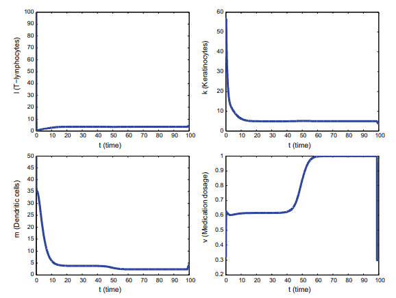
Further, only numerical investigation of optimal control $v_{*}(t)$ is possible. For the corresponding numerical calculations, the following values of the parameters and initial conditions of system (1) were used [3,11], as well as the control constraints (2):
$$
\begin{array}{llll}
\sigma=15.0 & \rho=3.6 & \beta=0.4 & \delta=0.005 \
\mu=0.01 & v=0.02 & \gamma_{1}=0.8 & \gamma_{2}=0.05 \
l_{0}=100.0 & k_{0}=40.0 & m_{0}=50.0 & \
v_{\min }=0.3 & T=100.0 & &
\end{array}
$$
The numerical calculations were carried out using the software “BOCOP 2.0.5” (see [1]), and are shown in Figs. 1 and $2 .$
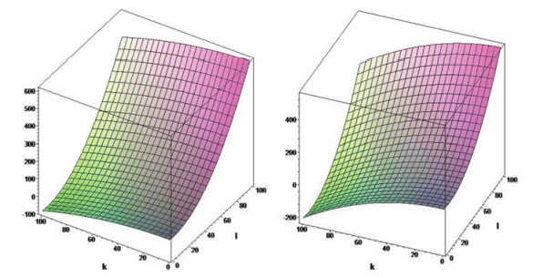
In Fig. 3 the surface $\Phi(l, k)$ is presented. It can be seen that positive values of the function $\Phi(l, k)$ in formula (10) in the region of variation of the variables $l$ and $k$ provide the admissibility of singular control $v_{\text {sing }}^{*}(t)$.
Physical optimal control $\tilde{v}{}(t)$ according to Figs. 1 and 2 describes the situation when, first there is the period of the psoriasis treatment with greatest intensity. Next, it is followed by the period of the treatment with a smooth decrease in the dose of the used medication from the greatest intensity to the lower intensity. Then, there is a period of the psoriasis treatment with lower intensity, and finally the switching occurs to the period of the treatment with greatest intensity. Also, we emphasize that in all performed numerical calculations, the optimal concentration of keratinocytes $k{}(t)$ decreases to the end $T$ to the level that is the minimal for the entire period $[0, T]$ of the psoriasis treatment (see Figs. 1 and 2 ).
数学分析代考
数学代写|数学分析代写Mathematical Analysis代考|Properties of the Switching Function
功能分析 $L(t)$ 导致以下引理的有效性。
引理 2 有这样一个值 $t_{0} \in[0, T)$ 在区间 $\left(t_{0}, T\right]$ 切换功能 $L(t)$ 是负数。
证明函数 $\psi_{1}(t), \psi_{2}(t), \psi_{3}(t)$ ,作为绝对连续解的分量 $\psi(t)$ 到系统 (5),也是绝对连续的。因此,由公式
(7) ,切换函数 $L(t)$ 也是绝对连续的,因此是连续函数。由于公式 (7) 和系统 (5) 的初始条件,它在 $t=T$
$$
L(T)=-(\beta+\delta)<0 .
$$
那么,连续函数符号的稳定性 $L(t)$ 产生所需的事实。这样就完成了证明。
推论 1 由引理 2 和公式 (6) 可知:
$$
v(t)=v_{\min }, \quad t \in\left(t_{0}, T\right] .
$$
现在,我们引入正常数:
$$
\alpha=\gamma_{2}^{-1}\left((\beta+\delta) \gamma_{1}-\delta \gamma_{2}\right), \quad \varepsilon=\alpha(\lambda-v)+\delta(\lambda-\mu)
$$
然后还有以下功能:
$$
g_{11}(t)=v(t)(\delta m(t)+\beta l(t))+v g_{21}(t)=\quad v(t) m(t)\left(\gamma_{1}(\delta k(t)-(\beta+\delta) l(t))+\delta(\mu-v)\right) g_{22}(t)
$$
数学代写|数学分析代写Mathematical Analysis代考|Numerical Results
此外,只有最优控制的数值研究 $v_{}(t)$ 是可能的。对于相应的数值计算,系统 (1) 的参数和初始条件的以下值被 使用 $[3,11]$ ,以及控制约束 (2): $$ \sigma=15.0 \quad \rho=3.6 \quad \beta=0.4 \quad \delta=0.005 \mu=0.01 \quad v=0.02 \quad \gamma_{1}=0.8 \quad \gamma_{2}=0.05 l_{0}=100.0 $$ 数值计算是使用软件”BOCOP 2.0.5″ (参见[1]) 进行的,如图 1 和图 2 所示。 1 和 2 . 在图 3 中的表面 $\Phi(l, k)$ 被呈现。可以看出函数的正值 $\Phi(l, k)$ 式 (10) 中变量的变化区域 $l$ 和 $k$ 提供单一控制的可 接受性 $v_{\text {sing }}^{}(t)$
物理优化控制 $\tilde{v}(t)$ 根据图。图1和图2描述了首先是牛皮癖治疗强度最大的时期的情况。接下来是治疗期间,所用 药物的剂量从最大强度平稳减少到较低强度。然后,有一个强度较低的银屑病治疗期,最后切换到强度最大的治 疗期。此外,我们强调在所有进行的数值计算中,角质形成细胞的最佳浓度 $k(t)$ 减少到最后 $T$ 到整个时期的最低 水平 $[0, T]$ 牛皮㿈治疗(见图1和 2 )。

统计代写请认准statistics-lab™. statistics-lab™为您的留学生涯保驾护航。
金融工程代写
金融工程是使用数学技术来解决金融问题。金融工程使用计算机科学、统计学、经济学和应用数学领域的工具和知识来解决当前的金融问题,以及设计新的和创新的金融产品。
非参数统计代写
非参数统计指的是一种统计方法,其中不假设数据来自于由少数参数决定的规定模型;这种模型的例子包括正态分布模型和线性回归模型。
广义线性模型代考
广义线性模型(GLM)归属统计学领域,是一种应用灵活的线性回归模型。该模型允许因变量的偏差分布有除了正态分布之外的其它分布。
术语 广义线性模型(GLM)通常是指给定连续和/或分类预测因素的连续响应变量的常规线性回归模型。它包括多元线性回归,以及方差分析和方差分析(仅含固定效应)。
有限元方法代写
有限元方法(FEM)是一种流行的方法,用于数值解决工程和数学建模中出现的微分方程。典型的问题领域包括结构分析、传热、流体流动、质量运输和电磁势等传统领域。
有限元是一种通用的数值方法,用于解决两个或三个空间变量的偏微分方程(即一些边界值问题)。为了解决一个问题,有限元将一个大系统细分为更小、更简单的部分,称为有限元。这是通过在空间维度上的特定空间离散化来实现的,它是通过构建对象的网格来实现的:用于求解的数值域,它有有限数量的点。边界值问题的有限元方法表述最终导致一个代数方程组。该方法在域上对未知函数进行逼近。[1] 然后将模拟这些有限元的简单方程组合成一个更大的方程系统,以模拟整个问题。然后,有限元通过变化微积分使相关的误差函数最小化来逼近一个解决方案。
tatistics-lab作为专业的留学生服务机构,多年来已为美国、英国、加拿大、澳洲等留学热门地的学生提供专业的学术服务,包括但不限于Essay代写,Assignment代写,Dissertation代写,Report代写,小组作业代写,Proposal代写,Paper代写,Presentation代写,计算机作业代写,论文修改和润色,网课代做,exam代考等等。写作范围涵盖高中,本科,研究生等海外留学全阶段,辐射金融,经济学,会计学,审计学,管理学等全球99%专业科目。写作团队既有专业英语母语作者,也有海外名校硕博留学生,每位写作老师都拥有过硬的语言能力,专业的学科背景和学术写作经验。我们承诺100%原创,100%专业,100%准时,100%满意。
随机分析代写
随机微积分是数学的一个分支,对随机过程进行操作。它允许为随机过程的积分定义一个关于随机过程的一致的积分理论。这个领域是由日本数学家伊藤清在第二次世界大战期间创建并开始的。
时间序列分析代写
随机过程,是依赖于参数的一组随机变量的全体,参数通常是时间。 随机变量是随机现象的数量表现,其时间序列是一组按照时间发生先后顺序进行排列的数据点序列。通常一组时间序列的时间间隔为一恒定值(如1秒,5分钟,12小时,7天,1年),因此时间序列可以作为离散时间数据进行分析处理。研究时间序列数据的意义在于现实中,往往需要研究某个事物其随时间发展变化的规律。这就需要通过研究该事物过去发展的历史记录,以得到其自身发展的规律。
回归分析代写
多元回归分析渐进(Multiple Regression Analysis Asymptotics)属于计量经济学领域,主要是一种数学上的统计分析方法,可以分析复杂情况下各影响因素的数学关系,在自然科学、社会和经济学等多个领域内应用广泛。
MATLAB代写
MATLAB 是一种用于技术计算的高性能语言。它将计算、可视化和编程集成在一个易于使用的环境中,其中问题和解决方案以熟悉的数学符号表示。典型用途包括:数学和计算算法开发建模、仿真和原型制作数据分析、探索和可视化科学和工程图形应用程序开发,包括图形用户界面构建MATLAB 是一个交互式系统,其基本数据元素是一个不需要维度的数组。这使您可以解决许多技术计算问题,尤其是那些具有矩阵和向量公式的问题,而只需用 C 或 Fortran 等标量非交互式语言编写程序所需的时间的一小部分。MATLAB 名称代表矩阵实验室。MATLAB 最初的编写目的是提供对由 LINPACK 和 EISPACK 项目开发的矩阵软件的轻松访问,这两个项目共同代表了矩阵计算软件的最新技术。MATLAB 经过多年的发展,得到了许多用户的投入。在大学环境中,它是数学、工程和科学入门和高级课程的标准教学工具。在工业领域,MATLAB 是高效研究、开发和分析的首选工具。MATLAB 具有一系列称为工具箱的特定于应用程序的解决方案。对于大多数 MATLAB 用户来说非常重要,工具箱允许您学习和应用专业技术。工具箱是 MATLAB 函数(M 文件)的综合集合,可扩展 MATLAB 环境以解决特定类别的问题。可用工具箱的领域包括信号处理、控制系统、神经网络、模糊逻辑、小波、仿真等。