如果你也在 怎样代写概率论Probability theory这个学科遇到相关的难题,请随时右上角联系我们的24/7代写客服。
概率论是与概率有关的数学分支。虽然有几种不同的概率解释,但概率论以严格的数学方式处理这一概念,通过一套公理来表达它。
statistics-lab™ 为您的留学生涯保驾护航 在代写概率论Probability theory方面已经树立了自己的口碑, 保证靠谱, 高质且原创的统计Statistics代写服务。我们的专家在代写概率论Probability theory代写方面经验极为丰富,各种代写概率论Probability theory相关的作业也就用不着说。
我们提供的概率论Probability theory及其相关学科的代写,服务范围广, 其中包括但不限于:
- Statistical Inference 统计推断
- Statistical Computing 统计计算
- Advanced Probability Theory 高等概率论
- Advanced Mathematical Statistics 高等数理统计学
- (Generalized) Linear Models 广义线性模型
- Statistical Machine Learning 统计机器学习
- Longitudinal Data Analysis 纵向数据分析
- Foundations of Data Science 数据科学基础
数学代写|概率论代写Probability theory代考|Estimation of Relative Permeability Function
The soil dry density has significant influence not only on the SWCC but also on other properties of unsaturated soil. In this section, the proposed SWCC model is applied to estimate the relative permeability function of unsaturated soil. The relative permeability function, $k_{r}$, is the ratio of the effective permeability to the saturated permeability for the unsaturated soil $k_{\mathrm{r}}=k_{\mathrm{w}} / k_{\mathrm{s}}$. Several statistical formulae have been proposed to estimate the relative permeability function from $S W C C$ equation by previous researchers. Fredlund et al. $[42,43]$ proposed using the FX equation to predict the coefficient of permeability for unsaturated soil. The formula has the following integration form:
$$
k_{\mathrm{r}}(\phi)=\Theta \frac{\int_{\phi}^{\phi_{0}} \frac{\theta(v)-\theta(\phi)}{v^{2}} \theta^{\prime}(v) \mathrm{d} v}{\int_{\phi_{s}}^{\phi_{0}} \frac{\theta(v)-\theta}{v^{2}} \theta^{\prime}(v) \mathrm{d} v}
$$
where $v$ is a dummy variable associated with the suction; $\varphi_{0}$ is the suction corresponding to complete dryness, $\varphi_{0}=10^{6} \mathrm{kPa} ; \varphi_{\mathrm{s}}$ is the suction corresponding to the initial saturated water content $\theta_{\mathrm{s}}$ and it has a small finite value, $\varphi_{\mathrm{s}}=0.001 \mathrm{kPa}$,
to avoid singularity in the integration; $\theta^{\prime}$ is the derivative of the volumetric water content function; $\Theta$ is the correction factor used here which can take tortuosity into consideration and increases the flexibility of the permeability estimation equation.
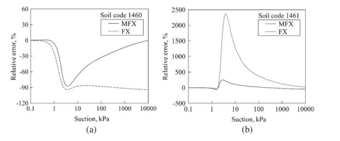
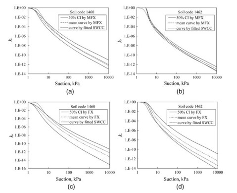
By using Eq. (2.9), both MFX and FX can be used to estimate $k_{\mathrm{r}}$ values. Figure $2.6$ presents the measured and estimated $k_{\mathrm{r}}$ values from MFX and FX for Berlin coarse sand, with the use of the fitting parameters shown in Table 2.4. The SWCC of each soil code was also computed by curve-fitting of Eq. (2.2), and then the SWCC was used in Eq. (2.9) to compute $k_{\mathrm{r}}$, denoted as “fitted curve” in Fig. 2.6. Comparing the fitted curve with the measured $k_{\mathrm{r}}$, it can be seen that the fitted curve does not perfectly agree with the measured data. This disagreement is suspected to be due to the error of measurements or the estimation model, that is, Eq. (2.9) in this case. In order to eliminate the effect of measurement error and model error, the fitted curve is used as a reference to compare with the estimated $k_{\mathrm{r}}$ by MFX and FX. It is found in Fig. $2.6$ that the MFX can well predict the $k_{\mathrm{r}}$ for the soils with different initial porosities, while the estimated $k_{\mathrm{r}}$ by FX deviates substantially from the “fitted curve”.
In order to clearly show the difference between the estimated $k_{\mathrm{r}}$ by MFX and FX, the “fitted curve” is used to compute the relative error of the $k_{\mathrm{r}}$ values. The relative error $(R E)$ is defined as:
$$
R E=\frac{k_{\mathrm{r}, \text { estimated }}-k_{\mathrm{r}, \text { fitted curve }}}{k_{\mathrm{r}, \text { fited curve }}} \times 100 \%
$$
where $k_{\mathrm{r}}$, estimated is the value estimated by the SWCC of MFX or FX and $k_{\mathrm{r}}$, fited curve is the value in the fitted curve. Figure $2.7$ depicts the relative error of $k_{\mathrm{r}}$ values estimated by the SWCCs of MFX and FX for Berlin coarse sand. It is clearly seen that the $R E$ value of $k_{\mathrm{r}}$ estimated by MFX is much smaller than that by FX for a wide range of suction.
数学代写|概率论代写Probability theory代考|Establishment of Relationships
Arya and Paris [14] presented a SWCC model that combined physical hypotheses with an empirical presentation. Based on the shape similarity between the SWCC and the cumulative PSD curve, the Arya and Paris (AP) model was established using the PSD and dry unit weight of a soil. The model considers the water flow paths in the soil as a bundle of capillary tubes and assumes that the size of the soil particles is related to the corresponding pore diameters of the capillary tubes.
Given a set of SWCC data for a soil sample (1) with a known initial void ratio $\left(e^{(1)}\right)$, the fitting SWCC can be obtained using the Fredlund and Xing empirical equation [17]:
$$
\theta_{\mathrm{w}}=\frac{\theta_{\mathrm{s}}}{\left{\ln \left[\exp (1)+(\varphi / a)^{n}\right]\right}^{m}}
$$
where $\theta_{\mathrm{s}}$ is the saturated volumetric water content; $a, n$ and $m$ are three adjustable parameters; and $\varphi$ is the matric suction of soil. The fitting results for the set of measured SWCC data can be written as $\left(\theta_{w}^{(1)}, \varphi^{(1)}\right)$. Using the dimensionless volumetric water content, $S=\theta_{\mathrm{w}} / \theta_{\mathrm{s}}$, Eq. (3.1) can be re-written as follows:
$$
S=\frac{1}{\left{\ln \left[\exp (1)+(\varphi / a)^{n}\right]\right}^{m}}
$$
The estimation of the $\operatorname{SWCC}\left(\theta_{\mathrm{w}}^{(2)}, \varphi^{(2)}\right)$ of a soil sample $(2)$ that has the same PSD curve as the sample (1) but a different initial void ratio $\left(e^{(2)}\right)$ is presented as follows.
数学代写|概率论代写Probability theory代考|Relationship of Volumetric Water Contents
The particle-size distribution curve is divided into $n$ fractions. The solid particles in each fraction are assumed to be of uniform particle size. Assembling all the fractions, a natural structure sample is formed. The dry density of the sample is assumed equal to that of each assemblage of the $n$ fractions.
The pore volume of each fraction per unit sample mass is given as follows:
$$
V_{\mathrm{v} i}=m_{\mathrm{si}} e / \rho_{\mathrm{s}} \quad i=1,2, \ldots, n
$$
where $V_{\mathrm{v} i}$ is the soil pore volume of the $i$ th fraction per unit sample mass; $m_{\mathrm{si}}$ is the soil particle mass of the $i$ th fraction per unit sample mass; $\rho_{\mathrm{s}}$ is the soil particle mass density; and $e$ is the initial void ratio. The first fraction of the assemblage has the smallest pore size.
It is assumed that soil water will first fill in the small pores in the soil at certain water contents. Thus, the volumetric water content of the soil sample when the pores of the $i$ th fraction are filled with water can be calculated by the accumulated pore volume:
$$
\theta_{\mathrm{w} i}=\sum_{j=1}^{j=i} V_{\mathrm{v} j} / V \quad i=1,2, \ldots, n
$$
where $V$ is the sample volume per unit sample mass.
Based on Eqs. (3.3) and (3.4), the volumetric water contents of two soil samples (1) and (2) satisfy the following relationship:
$$
\frac{\theta_{\mathrm{w} i}^{(2)}}{\theta_{\mathrm{w} i}^{(1)}}=\frac{e^{(2)} V^{(1)} \sum_{j=1}^{j=i} m_{\mathrm{s} j}^{(2)}}{e^{(1)} V^{(2)} \sum_{j=1}^{j=i} m_{\mathrm{s} j}^{(1)}}
$$
where $\theta_{\text {wi }}^{(1)}$ is the volumetric water content when the $i$ th soil pore is filled with water in soil sample (1) with initial void ratio $e^{(1)}$, and $\theta_{w i}^{(2)}$ is that of soil sample (2) with initial void ratio $e^{(2)}$.
Based on the PSD curve, the particle mass in each fraction is the same in both soil samples, that is, $m_{\mathrm{s} j}^{(2)}=m_{\mathrm{s} j}^{(1)}, j=1,2, \ldots, i$. Considering the phase relationships $\rho_{\mathrm{s}} V_{\mathrm{s}}=\rho_{d} V$ and $\rho_{d}=G_{s} \rho_{\mathrm{w}} /(1+e)$, the following equation can be obtained:
$$
\frac{V^{(2)}}{V^{(1)}}=\frac{1+e^{(2)}}{1+e^{(1)}}
$$
Thus, the ratio of the volumetric water content can be obtained by substituting Eqs. (3.6) into (3.5):
$$
\frac{\theta_{w i}^{(2)}}{\theta_{w i}^{(1)}}=\frac{e^{(2)}\left(1+e^{(1)}\right)}{e^{(1)}\left(1+e^{(2)}\right)}
$$
The volumetric water content of soil sample (2) can be estimated using the volumetric water content data of soil sample (1) and the initial void ratios.
概率论代考
数学代写|概率论代写Probability theory代考|Estimation of Relative Permeability Function
土壤干密度不仅对SWCC有显着影响,而且对非饱和土的其他性质也有显着影响。在本节中,所提出的 SWCC 模型用于估计非饱和土的相对渗透率函数。相对渗透率函数,ķr, 是非饱和土的有效渗透率与饱和渗透率之比ķr=ķ在/ķs. 已经提出了几个统计公式来估计相对渗透率函数小号在CC以前的研究人员的方程。弗雷德伦德等人。[42,43]建议使用 FX 方程来预测非饱和土壤的渗透系数。该公式具有以下积分形式:
ķr(φ)=θ∫φφ0θ(在)−θ(φ)在2θ′(在)d在∫φsφ0θ(在)−θ在2θ′(在)d在
在哪里在是与吸力相关的虚拟变量;披0是与完全干燥相对应的吸力,披0=106ķ磷一个;披s是对应于初始饱和含水量的吸力θs它有一个小的有限值,披s=0.001ķ磷一个,
避免集成中的奇异性;θ′是体积含水量函数的导数;θ是这里使用的修正系数,可以考虑曲折度,增加渗透率估计方程的灵活性。
通过使用方程式。(2.9),MFX和FX都可以用来估计ķr价值观。数字2.6呈现测量和估计的ķr柏林粗砂的 MFX 和 FX 值,使用表 2.4 中所示的拟合参数。每个土壤代码的 SWCC 也通过方程的曲线拟合计算。(2.2),然后在方程式中使用SWCC。(2.9) 计算ķr,在图 2.6 中表示为“拟合曲线”。将拟合曲线与测量曲线进行比较ķr,可以看出拟合曲线与实测数据并不完全吻合。这种不一致被怀疑是由于测量误差或估计模型,即方程。(2.9) 在这种情况下。为了消除测量误差和模型误差的影响,以拟合曲线作为参考,与估计值进行比较ķr通过 MFX 和 FX。它可以在图 3 中找到。2.6MFX 可以很好地预测ķr对于具有不同初始孔隙度的土壤,而估计的ķr由 FX 大幅偏离“拟合曲线”。
为了清楚地显示估计之间的差异ķr通过 MFX 和 FX,“拟合曲线”用于计算相对误差ķr价值观。相对误差(R和)定义为:
R和=ķr, 估计的 −ķr, 拟合曲线 ķr, 拟合曲线 ×100%
在哪里ķr, 估计是 MFX 或 FX 的 SWCC 估计的值和ķr, 拟合曲线是拟合曲线中的值。数字2.7描述了相对误差ķr柏林粗砂的 MFX 和 FX 的 SWCC 估计的值。可以清楚地看出,R和的价值ķr对于大范围的吸力,MFX 估算的比 FX 估算的要小得多。
数学代写|概率论代写Probability theory代考|Establishment of Relationships
Arya 和 Paris [14] 提出了一个 SWCC 模型,该模型将物理假设与经验演示相结合。基于 SWCC 和累积 PSD 曲线的形状相似性,利用土壤的 PSD 和干单位重量建立 Arya 和 Paris (AP) 模型。该模型将土壤中的水流路径视为一束毛细管,并假设土壤颗粒的大小与相应的毛细管孔径有关。
给定具有已知初始空隙比的土壤样品 (1) 的一组 SWCC 数据(和(1)),拟合 SWCC 可以使用 Fredlund 和 Xing 经验方程 [17] 获得:
\theta_{\mathrm{w}}=\frac{\theta_{\mathrm{s}}}{\left{\ln \left[\exp (1)+(\varphi / a)^{n}\right ]\右}^{m}}\theta_{\mathrm{w}}=\frac{\theta_{\mathrm{s}}}{\left{\ln \left[\exp (1)+(\varphi / a)^{n}\right ]\右}^{m}}
在哪里θs是饱和体积含水量;一个,n和米是三个可调参数;和披是土壤的基质吸力。测量的 SWCC 数据集的拟合结果可以写为(θ在(1),披(1)). 使用无量纲的体积含水量,小号=θ在/θs, 方程。(3.1)式可改写如下:
S=\frac{1}{\left{\ln \left[\exp (1)+(\varphi / a)^{n}\right]\right}^{m}}S=\frac{1}{\left{\ln \left[\exp (1)+(\varphi / a)^{n}\right]\right}^{m}}
的估计SWCC(θ在(2),披(2))土壤样品(2)具有与样品 (1) 相同的 PSD 曲线,但初始空隙率不同(和(2))介绍如下。
数学代写|概率论代写Probability theory代考|Relationship of Volumetric Water Contents
粒度分布曲线分为n分数。假设每个部分中的固体颗粒具有均匀的粒径。组装所有的部分,形成一个自然的结构样本。假设样品的干密度等于每个组合的干密度n分数。
每单位样品质量的每个馏分的孔体积如下:
在在一世=米s一世和/ρs一世=1,2,…,n
在哪里在在一世是土壤的孔隙体积一世每单位样品质量的分数;米s一世是土壤颗粒质量一世每单位样品质量的分数;ρs是土壤颗粒质量密度;和和是初始空隙率。组合的第一部分具有最小的孔径。
假设土壤水分在一定的含水量下会首先填满土壤中的小孔隙。因此,土壤样品的体积含水量一世第 th 部分充满水可以通过累积的孔隙体积计算:
θ在一世=∑j=1j=一世在在j/在一世=1,2,…,n
在哪里在是每单位样品质量的样品体积。
基于方程式。(3.3)和(3.4),两个土壤样品(1)和(2)的体积含水量满足以下关系:
θ在一世(2)θ在一世(1)=和(2)在(1)∑j=1j=一世米sj(2)和(1)在(2)∑j=1j=一世米sj(1)
在哪里θ无线 (1)是体积含水量,当一世土样 (1) 中的土壤孔隙充满水,初始孔隙比和(1), 和θ在一世(2)是具有初始孔隙比的土壤样品 (2)和(2).
根据 PSD 曲线,两个土壤样品中每个部分的颗粒质量相同,即米sj(2)=米sj(1),j=1,2,…,一世. 考虑相位关系ρs在s=ρd在和ρd=Gsρ在/(1+和),可以得到以下等式:
在(2)在(1)=1+和(2)1+和(1)
因此,体积含水量的比值可以通过代入方程得到。(3.6)到(3.5):
θ在一世(2)θ在一世(1)=和(2)(1+和(1))和(1)(1+和(2))
土壤样品 (2) 的体积含水量可以使用土壤样品 (1) 的体积含水量数据和初始空隙率来估计。

统计代写请认准statistics-lab™. statistics-lab™为您的留学生涯保驾护航。
金融工程代写
金融工程是使用数学技术来解决金融问题。金融工程使用计算机科学、统计学、经济学和应用数学领域的工具和知识来解决当前的金融问题,以及设计新的和创新的金融产品。
非参数统计代写
非参数统计指的是一种统计方法,其中不假设数据来自于由少数参数决定的规定模型;这种模型的例子包括正态分布模型和线性回归模型。
广义线性模型代考
广义线性模型(GLM)归属统计学领域,是一种应用灵活的线性回归模型。该模型允许因变量的偏差分布有除了正态分布之外的其它分布。
术语 广义线性模型(GLM)通常是指给定连续和/或分类预测因素的连续响应变量的常规线性回归模型。它包括多元线性回归,以及方差分析和方差分析(仅含固定效应)。
有限元方法代写
有限元方法(FEM)是一种流行的方法,用于数值解决工程和数学建模中出现的微分方程。典型的问题领域包括结构分析、传热、流体流动、质量运输和电磁势等传统领域。
有限元是一种通用的数值方法,用于解决两个或三个空间变量的偏微分方程(即一些边界值问题)。为了解决一个问题,有限元将一个大系统细分为更小、更简单的部分,称为有限元。这是通过在空间维度上的特定空间离散化来实现的,它是通过构建对象的网格来实现的:用于求解的数值域,它有有限数量的点。边界值问题的有限元方法表述最终导致一个代数方程组。该方法在域上对未知函数进行逼近。[1] 然后将模拟这些有限元的简单方程组合成一个更大的方程系统,以模拟整个问题。然后,有限元通过变化微积分使相关的误差函数最小化来逼近一个解决方案。
tatistics-lab作为专业的留学生服务机构,多年来已为美国、英国、加拿大、澳洲等留学热门地的学生提供专业的学术服务,包括但不限于Essay代写,Assignment代写,Dissertation代写,Report代写,小组作业代写,Proposal代写,Paper代写,Presentation代写,计算机作业代写,论文修改和润色,网课代做,exam代考等等。写作范围涵盖高中,本科,研究生等海外留学全阶段,辐射金融,经济学,会计学,审计学,管理学等全球99%专业科目。写作团队既有专业英语母语作者,也有海外名校硕博留学生,每位写作老师都拥有过硬的语言能力,专业的学科背景和学术写作经验。我们承诺100%原创,100%专业,100%准时,100%满意。
随机分析代写
随机微积分是数学的一个分支,对随机过程进行操作。它允许为随机过程的积分定义一个关于随机过程的一致的积分理论。这个领域是由日本数学家伊藤清在第二次世界大战期间创建并开始的。
时间序列分析代写
随机过程,是依赖于参数的一组随机变量的全体,参数通常是时间。 随机变量是随机现象的数量表现,其时间序列是一组按照时间发生先后顺序进行排列的数据点序列。通常一组时间序列的时间间隔为一恒定值(如1秒,5分钟,12小时,7天,1年),因此时间序列可以作为离散时间数据进行分析处理。研究时间序列数据的意义在于现实中,往往需要研究某个事物其随时间发展变化的规律。这就需要通过研究该事物过去发展的历史记录,以得到其自身发展的规律。
回归分析代写
多元回归分析渐进(Multiple Regression Analysis Asymptotics)属于计量经济学领域,主要是一种数学上的统计分析方法,可以分析复杂情况下各影响因素的数学关系,在自然科学、社会和经济学等多个领域内应用广泛。
MATLAB代写
MATLAB 是一种用于技术计算的高性能语言。它将计算、可视化和编程集成在一个易于使用的环境中,其中问题和解决方案以熟悉的数学符号表示。典型用途包括:数学和计算算法开发建模、仿真和原型制作数据分析、探索和可视化科学和工程图形应用程序开发,包括图形用户界面构建MATLAB 是一个交互式系统,其基本数据元素是一个不需要维度的数组。这使您可以解决许多技术计算问题,尤其是那些具有矩阵和向量公式的问题,而只需用 C 或 Fortran 等标量非交互式语言编写程序所需的时间的一小部分。MATLAB 名称代表矩阵实验室。MATLAB 最初的编写目的是提供对由 LINPACK 和 EISPACK 项目开发的矩阵软件的轻松访问,这两个项目共同代表了矩阵计算软件的最新技术。MATLAB 经过多年的发展,得到了许多用户的投入。在大学环境中,它是数学、工程和科学入门和高级课程的标准教学工具。在工业领域,MATLAB 是高效研究、开发和分析的首选工具。MATLAB 具有一系列称为工具箱的特定于应用程序的解决方案。对于大多数 MATLAB 用户来说非常重要,工具箱允许您学习和应用专业技术。工具箱是 MATLAB 函数(M 文件)的综合集合,可扩展 MATLAB 环境以解决特定类别的问题。可用工具箱的领域包括信号处理、控制系统、神经网络、模糊逻辑、小波、仿真等。