如果你也在 怎样代写线性代数linear algebra这个学科遇到相关的难题,请随时右上角联系我们的24/7代写客服。
线性代数是平坦的微分几何,在流形的切线空间中服务。时空的电磁对称性是由洛伦兹变换表达的,线性代数的大部分历史就是洛伦兹变换的历史。
statistics-lab™ 为您的留学生涯保驾护航 在代写线性代数linear algebra方面已经树立了自己的口碑, 保证靠谱, 高质且原创的统计Statistics代写服务。我们的专家在代写线性代数linear algebra代写方面经验极为丰富,各种代写线性代数linear algebra相关的作业也就用不着说。
我们提供的线性代数linear algebra及其相关学科的代写,服务范围广, 其中包括但不限于:
- Statistical Inference 统计推断
- Statistical Computing 统计计算
- Advanced Probability Theory 高等概率论
- Advanced Mathematical Statistics 高等数理统计学
- (Generalized) Linear Models 广义线性模型
- Statistical Machine Learning 统计机器学习
- Longitudinal Data Analysis 纵向数据分析
- Foundations of Data Science 数据科学基础
数学代写|线性代数代写linear algebra代考|Diffusion Welding and Heat States
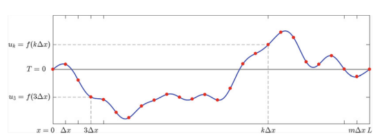
In this section, we begin a deeper look into the mathematics for the diffusion welding application discussed in Chapter 1. Recall that diffusion welding can be used to adjoin several smaller rods into a single longer rod, leaving the final rod just after welding with varying temperature along the rod but with the ends having the same temperature. Recall that we measure the temperature along the rod and obtain a heat signature like the one seen in Figure $1.4$ of Chapter 1. Recall also, that the heat signature shows the temperature difference from the temperature at the ends of the rod. Thus, the initial signature (along with any subsequent signature) will show values of 0 at the ends.
The heat signature along the rod can be described by a function $f:[0, L] \rightarrow \mathbb{R}$, where $L$ is the length of the rod and $f(0)=f(L)=0$. The quantity $f(x)$ is the temperature difference on the rod at a position $x$ in the interval $[0, L]$. Because we are detecting and storing heat measurements along the rod, we are only able to collect finitely many such measurements. Thus, we discretize the heat signature $f$ by sampling at only $m$ locations along the bar. If we space the $m$ sampling locations equally, then for $\Delta x=\frac{L}{m+1}$, we can choose the sampling locations to be $\Delta x, 2 \Delta x, \ldots, m \Delta x$. Since the heat measurement is zero (and fixed) at the endpoints we do not need to sample there. The set of discrete heat measurements at a given time is called a heat state, as opposed to a heat signature, which, as discussed earlier, is defined at every point along the rod. We can record the heat state as the vector
$$
u=\left[u_{0}, u_{1}, u_{2}, \ldots, u_{m}, u_{m+1}\right]=[0, f(\Delta x), f(2 \Delta x), \ldots, f(m \Delta x), 0]
$$
Here, if $u_{j}=f(x)$ for some $x \in[0, L]$ then $u_{j+1}=f(x+\Delta x)$ and $u_{j-1}=f(x-\Delta x)$. Figure $2.15$ shows a (continuous) heat signature as a solid blue curve and the corresponding measured (discretized) heat state indicated by the regularly sampled points marked as circles.
数学代写|线性代数代写linear algebra代考|Function Spaces
We have seen that the set of discretized heat states of the preceding example forms a vector space. These discretized heat states can be viewed as real-valued functions on the set of $m+2$ points that are the sampling locations along the rod. In fact, function spaces such as $H_{m}(\mathbb{R})$ are very common and useful constructs for solving many physical problems. The following are some such function spaces.
Example 2.4.1 Let $\mathcal{F}={f: \mathbb{R} \rightarrow \mathbb{R}}$, the set of all functions whose domain is $\mathbb{R}$ and whose range consists of only real numbers.
We define addition and scalar multiplication (on functions) pointwise. That is, given two functions $f$ and $g$ and a real scalar $\alpha$, we define the sum $f+g$ by $(f+g)(x):=f(x)+g(x)$ and the scalar product $\alpha f$ by $(\alpha f)(x):=\alpha \cdot(f(x)) .(\mathcal{F},+, \cdot)$ is a vector space with scalars taken from $\mathbb{R}$.
Proof. Let $f, g, h \in \mathcal{F}$ and $\alpha, \beta \in \mathbb{R}$. We verify the 10 properties of Definition $2.3 .5$.
- Since $f: \mathbb{R} \rightarrow \mathbb{R}$ and $g: \mathbb{R} \rightarrow \mathbb{R}$ and based on the definition of addition, $f+g: \mathbb{R} \rightarrow \mathbb{R}$. So $f+g \in \mathcal{F}$ and $\mathcal{F}$ is closed over addition.
- Similarly, $\mathcal{F}$ is closed under scalar multiplication.
- Addition is commutative since
$$
\begin{aligned}
(f+g)(x) &=f(x)+g(x) \
&=g(x)+f(x) \
&=(g+f)(x)
\end{aligned}
$$
So, $f+g=g+f$ - And, addition associative because
$$
\begin{aligned}
((f+g)+h)(x) &=(f+g)(x)+h(x) \
&=(f(x)+g(x))+h(x) \
&=f(x)+(g(x)+h(x)) \
&=f(x)+(g+h)(x) \
&=(f+(g+h))(x)
\end{aligned}
$$
So $(f+g)+h=f+(g+h)$. - We see, also, that scalar multiplication is associative. Indeed,
$$
(\alpha \cdot(\beta \cdot f))(x)=(\alpha \cdot(\beta \cdot f(x)))=(\alpha \beta) f(x)=((\alpha \beta) \cdot f)(x)
$$
So $\alpha \cdot(\beta \cdot f)=(\alpha \beta) \cdot f$
数学代写|线性代数代写linear algebra代考|Matrix Spaces
A matrix is an array of real numbers arranged in a rectangular grid, for example, let
$$
A=\left(\begin{array}{lll}
1 & 2 & 3 \
5 & 7 & 9
\end{array}\right)
$$
The matrix $A$ has 2 rows (horizontal) and 3 columns (vertical), so we say it is a $2 \times 3$ matrix. In general, a matrix $B$ with $m$ rows and $n$ columns is called an $m \times n$ matrix. We say the dimensions of the matrix are $m$ and $n$.
Any two matrices with the same dimensions are added together by adding their entries entry-wise. A matrix is multiplied by a scalar by multiplying all of its entries by that scalar (that is, multiplication of a matrix by a scalar is also an entry-wise operation, as in Example 2.3.8).
Example 2.4.6 Let
$$
A=\left(\begin{array}{lll}
1 & 2 & 3 \
5 & 7 & 9
\end{array}\right), B=\left(\begin{array}{ccc}
1 & 0 & 1 \
-2 & 1 & 0
\end{array}\right), \text { and } C=\left(\begin{array}{ll}
1 & 2 \
3 & 5
\end{array}\right)
$$
Then
$$
A+B=\left(\begin{array}{lll}
2 & 2 & 4 \
3 & 8 & 9
\end{array}\right) \text {, }
$$
but since $A \in \mathcal{M}{2 \times 3}$ and $C \in \mathcal{M}{2 \times 2}$, the definition of matrix addition does not work to compute $A+C$. That is, $A+C$ is undefined.
Using the definition of scalar multiplication, we get
$$
3 \cdot A=\left(\begin{array}{lll}
3(1) & 3(2) & 3(3) \
3(5) & 3(7) & 3(9)
\end{array}\right)=\left(\begin{array}{ccc}
3 & 6 & 9 \
15 & 21 & 27
\end{array}\right)
$$
With this understanding of operations on matrices, we can now discuss $\left(\mathcal{M}_{m \times n},+, \cdot\right)$ as a vector space over $\mathbb{R}$.
线性代数代考
数学代写|线性代数代写linear algebra代考|Diffusion Welding and Heat States
在本节中,我们开始深入研究第 1 章中讨论的扩散焊接应用的数学。回想一下,扩散焊接可用于将几根较小的焊条连接成一根较长的焊条,在焊接后以不同的温度留下最终焊条沿着杆,但两端具有相同的温度。回想一下,我们沿棒测量温度并获得如图所示的热特征1.4第 1 章。还记得,热特征显示与棒末端温度的温差。因此,初始签名(以及任何后续签名)将在末尾显示 0 值。
沿杆的热特征可以用函数来描述F:[0,大号]→R, 在哪里大号是杆的长度和F(0)=F(大号)=0. 数量F(X)是杆上某一位置的温差X在区间[0,大号]. 因为我们沿着棒检测和存储热量测量值,所以我们只能收集有限多个这样的测量值。因此,我们离散化热特征F通过仅抽样米沿着酒吧的位置。如果我们将米平均采样位置,然后对于ΔX=大号米+1,我们可以选择采样位置为ΔX,2ΔX,…,米ΔX. 由于在端点处热量测量为零(并且是固定的),我们不需要在那里采样。在给定时间的一组离散热测量值称为热状态,而不是热特征,如前所述,热特征定义在棒的每个点上。我们可以将热状态记录为向量
在=[在0,在1,在2,…,在米,在米+1]=[0,F(ΔX),F(2ΔX),…,F(米ΔX),0]
在这里,如果在j=F(X)对于一些X∈[0,大号]然后在j+1=F(X+ΔX)和在j−1=F(X−ΔX). 数字2.15将(连续)热特征显示为实心蓝色曲线,以及由标记为圆圈的规则采样点指示的相应测量(离散)热状态。
数学代写|线性代数代写linear algebra代考|Function Spaces
我们已经看到,前面示例的离散化热状态集形成了一个向量空间。这些离散化的热态可以看作是集合上的实值函数米+2是沿杆的采样位置的点。事实上,功能空间如H米(R)是解决许多物理问题的非常常见和有用的结构。以下是一些这样的功能空间。
示例 2.4.1 让F=F:R→R, 域为的所有函数的集合R并且其范围仅由实数组成。
我们逐点定义加法和标量乘法(在函数上)。也就是说,给定两个函数F和G和一个真正的标量一个,我们定义总和F+G经过(F+G)(X):=F(X)+G(X)和标量积一个F经过(一个F)(X):=一个⋅(F(X)).(F,+,⋅)是一个向量空间,其标量取自R.
证明。让F,G,H∈F和一个,b∈R. 我们验证定义的 10 个属性2.3.5.
- 自从F:R→R和G:R→R并基于加法的定义,F+G:R→R. 所以F+G∈F和F加法结束。
- 相似地,F在标量乘法下是闭合的。
- 加法是可交换的,因为
(F+G)(X)=F(X)+G(X) =G(X)+F(X) =(G+F)(X)
所以,F+G=G+F - 并且,加法关联因为
((F+G)+H)(X)=(F+G)(X)+H(X) =(F(X)+G(X))+H(X) =F(X)+(G(X)+H(X)) =F(X)+(G+H)(X) =(F+(G+H))(X)
所以(F+G)+H=F+(G+H). - 我们还看到,标量乘法是关联的。的确,
(一个⋅(b⋅F))(X)=(一个⋅(b⋅F(X)))=(一个b)F(X)=((一个b)⋅F)(X)
所以一个⋅(b⋅F)=(一个b)⋅F
数学代写|线性代数代写linear algebra代考|Matrix Spaces
矩阵是排列在矩形网格中的实数数组,例如,让
一个=(123 579)
矩阵一个有 2 行(水平)和 3 列(垂直),所以我们说它是2×3矩阵。一般来说,矩阵乙和米行和n列称为米×n矩阵。我们说矩阵的维度是米和n.
任何两个具有相同维度的矩阵通过逐项添加它们的条目来相加。通过将矩阵的所有条目乘以该标量,矩阵乘以标量(即,矩阵乘以标量也是逐项操作,如示例 2.3.8 中所示)。
示例 2.4.6 让
一个=(123 579),乙=(101 −210), 和 C=(12 35)
然后
一个+乙=(224 389),
但是由于一个∈米2×3和C∈米2×2, 矩阵加法的定义对计算不起作用一个+C. 那是,一个+C未定义。
使用标量乘法的定义,我们得到
3⋅一个=(3(1)3(2)3(3) 3(5)3(7)3(9))=(369 152127)
有了对矩阵运算的理解,我们现在可以讨论(米米×n,+,⋅)作为一个向量空间R.

统计代写请认准statistics-lab™. statistics-lab™为您的留学生涯保驾护航。
金融工程代写
金融工程是使用数学技术来解决金融问题。金融工程使用计算机科学、统计学、经济学和应用数学领域的工具和知识来解决当前的金融问题,以及设计新的和创新的金融产品。
非参数统计代写
非参数统计指的是一种统计方法,其中不假设数据来自于由少数参数决定的规定模型;这种模型的例子包括正态分布模型和线性回归模型。
广义线性模型代考
广义线性模型(GLM)归属统计学领域,是一种应用灵活的线性回归模型。该模型允许因变量的偏差分布有除了正态分布之外的其它分布。
术语 广义线性模型(GLM)通常是指给定连续和/或分类预测因素的连续响应变量的常规线性回归模型。它包括多元线性回归,以及方差分析和方差分析(仅含固定效应)。
有限元方法代写
有限元方法(FEM)是一种流行的方法,用于数值解决工程和数学建模中出现的微分方程。典型的问题领域包括结构分析、传热、流体流动、质量运输和电磁势等传统领域。
有限元是一种通用的数值方法,用于解决两个或三个空间变量的偏微分方程(即一些边界值问题)。为了解决一个问题,有限元将一个大系统细分为更小、更简单的部分,称为有限元。这是通过在空间维度上的特定空间离散化来实现的,它是通过构建对象的网格来实现的:用于求解的数值域,它有有限数量的点。边界值问题的有限元方法表述最终导致一个代数方程组。该方法在域上对未知函数进行逼近。[1] 然后将模拟这些有限元的简单方程组合成一个更大的方程系统,以模拟整个问题。然后,有限元通过变化微积分使相关的误差函数最小化来逼近一个解决方案。
tatistics-lab作为专业的留学生服务机构,多年来已为美国、英国、加拿大、澳洲等留学热门地的学生提供专业的学术服务,包括但不限于Essay代写,Assignment代写,Dissertation代写,Report代写,小组作业代写,Proposal代写,Paper代写,Presentation代写,计算机作业代写,论文修改和润色,网课代做,exam代考等等。写作范围涵盖高中,本科,研究生等海外留学全阶段,辐射金融,经济学,会计学,审计学,管理学等全球99%专业科目。写作团队既有专业英语母语作者,也有海外名校硕博留学生,每位写作老师都拥有过硬的语言能力,专业的学科背景和学术写作经验。我们承诺100%原创,100%专业,100%准时,100%满意。
随机分析代写
随机微积分是数学的一个分支,对随机过程进行操作。它允许为随机过程的积分定义一个关于随机过程的一致的积分理论。这个领域是由日本数学家伊藤清在第二次世界大战期间创建并开始的。
时间序列分析代写
随机过程,是依赖于参数的一组随机变量的全体,参数通常是时间。 随机变量是随机现象的数量表现,其时间序列是一组按照时间发生先后顺序进行排列的数据点序列。通常一组时间序列的时间间隔为一恒定值(如1秒,5分钟,12小时,7天,1年),因此时间序列可以作为离散时间数据进行分析处理。研究时间序列数据的意义在于现实中,往往需要研究某个事物其随时间发展变化的规律。这就需要通过研究该事物过去发展的历史记录,以得到其自身发展的规律。
回归分析代写
多元回归分析渐进(Multiple Regression Analysis Asymptotics)属于计量经济学领域,主要是一种数学上的统计分析方法,可以分析复杂情况下各影响因素的数学关系,在自然科学、社会和经济学等多个领域内应用广泛。
MATLAB代写
MATLAB 是一种用于技术计算的高性能语言。它将计算、可视化和编程集成在一个易于使用的环境中,其中问题和解决方案以熟悉的数学符号表示。典型用途包括:数学和计算算法开发建模、仿真和原型制作数据分析、探索和可视化科学和工程图形应用程序开发,包括图形用户界面构建MATLAB 是一个交互式系统,其基本数据元素是一个不需要维度的数组。这使您可以解决许多技术计算问题,尤其是那些具有矩阵和向量公式的问题,而只需用 C 或 Fortran 等标量非交互式语言编写程序所需的时间的一小部分。MATLAB 名称代表矩阵实验室。MATLAB 最初的编写目的是提供对由 LINPACK 和 EISPACK 项目开发的矩阵软件的轻松访问,这两个项目共同代表了矩阵计算软件的最新技术。MATLAB 经过多年的发展,得到了许多用户的投入。在大学环境中,它是数学、工程和科学入门和高级课程的标准教学工具。在工业领域,MATLAB 是高效研究、开发和分析的首选工具。MATLAB 具有一系列称为工具箱的特定于应用程序的解决方案。对于大多数 MATLAB 用户来说非常重要,工具箱允许您学习和应用专业技术。工具箱是 MATLAB 函数(M 文件)的综合集合,可扩展 MATLAB 环境以解决特定类别的问题。可用工具箱的领域包括信号处理、控制系统、神经网络、模糊逻辑、小波、仿真等。