如果你也在 怎样代写编码理论Coding Theory这个学科遇到相关的难题,请随时右上角联系我们的24/7代写客服。
编码理论是研究编码的属性和它们各自对特定应用的适用性。编码被用于数据压缩、密码学、错误检测和纠正、数据传输和数据存储。各种科学学科,如信息论、电气工程、数学、语言学和计算机科学,都对编码进行了研究,目的是设计高效和可靠的数据传输方法。这通常涉及消除冗余和纠正或检测传输数据中的错误。
statistics-lab™ 为您的留学生涯保驾护航 在代写编码理论Coding Theory方面已经树立了自己的口碑, 保证靠谱, 高质且原创的统计Statistics代写服务。我们的专家在代写编码理论Coding Theory代写方面经验极为丰富,各种代写编码理论Coding Theory相关的作业也就用不着说。
我们提供的编码理论Coding Theory及其相关学科的代写,服务范围广, 其中包括但不限于:
- Statistical Inference 统计推断
- Statistical Computing 统计计算
- Advanced Probability Theory 高等概率论
- Advanced Mathematical Statistics 高等数理统计学
- (Generalized) Linear Models 广义线性模型
- Statistical Machine Learning 统计机器学习
- Longitudinal Data Analysis 纵向数据分析
- Foundations of Data Science 数据科学基础
数学代写|编码理论作业代写Coding Theory代考|Encoding of Convolutional Codes
The easiest way to introduce convolutional codes is by means of a specific example. Consider the convolutional encoder depicted in Figure 3.1. Information bits are shifted into a register of length $m=2$, i.e. a register with two binary memory elements. The output sequence results from multiplexing the two sequences denoted by $\mathbf{b}^{(1)}$ and $\mathbf{b}^{(2)}$. Each output bit is generated by modulo 2 addition of the current input bit and some symbols of the register contents. For instance, the information sequence $\mathbf{u}=(1,1,0,1,0,0, \ldots)$ will be encoded to $\mathbf{b}^{(1)}=(1,0,0,0,1,1, \ldots)$ and $\mathbf{b}^{(2)}=(1,1,1,0,0,1, \ldots)$. The generated code sequence after multiplexing of $\mathbf{b}^{(1)}$ and $\mathbf{b}^{(2)}$ is $\mathbf{b}=(1,1,0,1,0,1,0,0,1,0,1,1, \ldots)$.
A convolutional encoder is a linear sequential circuit and therefore a Linear TimeInvariant (LTI) system. It is well known that an LTI system is completely characterized
by its impulse response. Let us therefore investigate the two impulse responses of this particular encoder. The information sequence $\mathbf{u}=1,0,0,0, \ldots$ results in the output $\mathbf{b}^{(1)}=$ $(1,1,1,0, \ldots)$ and $\mathbf{b}^{(2)}=(1,0,1,0, \ldots)$, i.e. we obtain the generator impulse responses $\mathbf{g}^{(1)}=(1,1,1,0, \ldots)$ and $\mathbf{g}^{(2)}=(1,0,1,0, \ldots)$ respectively. These generator impulse responses are helpful for calculating the output sequences for an arbitrary input sequence
$$
\begin{aligned}
&b_{i}^{(1)}=\sum_{l=0}^{m} u_{i-l} g_{l}^{(1)} \leftrightarrow \mathbf{b}^{(1)}=\mathbf{u} * \mathbf{g}^{(1)} \
&b_{i}^{(2)}=\sum_{l=0}^{m} u_{i-l} g_{l}^{(2)} \leftrightarrow \mathbf{b}^{(2)}=\mathbf{u} * \mathbf{g}^{(2)}
\end{aligned}
$$
The generating equations for $\mathbf{b}^{(1)}$ and $\mathbf{b}^{(2)}$ can be regarded as convolutions of the input sequence with the generator impulse responses $\mathrm{g}^{(1)}$ and $\mathrm{g}^{(2)}$. The code $\mathrm{B}$ generated by this encoder is the set of all output sequences $\mathbf{b}$ that can be produced by convolution of arbitrary input sequence $\mathbf{u}$ with the generator impulse responses. This explains the name convolutional codes.
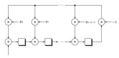
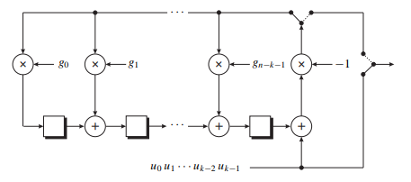
The general encoder of a rate $R=k / n$ convolutional code is depicted in Figure 3.2. Each input corresponds to a shift register, i.e. each information sequence is shifted into its own register. In contrast to block codes, the $i$ th code block $\mathbf{b}{i}=b{i}^{1}, b_{i}^{2}, \ldots, b_{i}^{n}$ of a convolutional code sequence $\mathbf{b}=\mathbf{b}{0}, \mathbf{b}{1}, \ldots$ is a linear function of several information blocks $\mathbf{u}{j}=u{j}^{1}, u_{j}^{2}, \ldots, u_{j}^{k}$ with $j \in{i-m, \ldots, i}$ and not only of $\mathbf{b}_{i}$. The integer $m$
denotes the memory of the encoder. The $k$ encoder registers do not necessarily have the same length. We denote the number of memory elements of the $l$ th register by $v_{l}$. The $n$ output sequences may depend on any of the $k$ registers. Thus, we require $k \times n$ impulse responses to characterise the encoding. If the shift registers are feedforward registers, i.e. they have no feedback, than the corresponding generator impulse responses $\mathbf{g}{l}^{(j)}$ are limited to length $v{l}+1$. For this reason, $v_{l}$ is often called the constraint length of the lth input sequence. The memory $m$ of the encoder is
$$
m=\max {l} v{l} .
$$
数学代写|编码理论作业代写Coding Theory代考|Generator Matrix in the Time Domain
Similarly to linear block codes, the encoding procedure can be described as a multiplication of the information sequence with a generator matrix $\mathbf{b}=\mathbf{u G}$. However, the information sequence $\mathbf{u}$ and the code sequence $\mathbf{b}$ are semi-infinite. Therefore, the generator matrix of a convolutional code also has a semi-infinite structure. It is constructed from $k \times n$ submatrices $\mathbf{G}{i}$ according to Figure $3.5$, where the elements of the submatrices are the coefficients from the generator impulse responses. For instance, for the encoder in Figure $3.1$ we obtain $$ \begin{aligned} &\mathbf{G}{0}=\left(g_{0}^{(1)}, g_{0}^{(2)}\right)=(11) \
&\mathbf{G}{1}=\left(g{1}^{(1)}, g_{1}^{(2)}\right)=\left(\begin{array}{ll}
1 & 0)
\end{array}\right. \
&\mathbf{G}{2}=\left(g{2}^{(1)}, g_{2}^{(2)}\right)=\left(\begin{array}{ll}
1 & 1
\end{array}\right)
\end{aligned}
$$
Finally, the generator matrix is
$$
\mathbf{G}=\left(\begin{array}{ccccccc}
\mathbf{G}{0} & \mathbf{G}{1} & \ldots & \mathbf{G}{m} & \mathbf{0} & \mathbf{0} & \ldots \ \mathbf{0} & \mathbf{G}{0} & \mathbf{G}{1} & \ldots & \mathbf{G}{m} & \mathbf{0} & \ldots \
\mathbf{0} & \mathbf{0} & \mathbf{G}{0} & \mathbf{G}{1} & \ldots & \mathbf{G}_{m} & \ldots \
\mathbf{0} & \mathbf{0} & \mathbf{0} & \ddots & \ddots & & \ddots
\end{array}\right)=\left(\begin{array}{cccccc}
11 & 10 & 11 & 00 & 00 & \ldots \
00 & 11 & 10 & 11 & 00 & \ldots \
00 & 00 & 11 & 10 & 11 & \ldots \
00 & 00 & 00 & \ddots & & \ddots
\end{array}\right) .
$$
With this generator matrix we can express the encoding of an information sequence, for instance $\mathbf{u}=(1,1,0,1,0,0, \ldots)$, by a matrix multiplication
$$
\begin{aligned}
\mathbf{b} &=\mathbf{u G}=(1,1,0,1,0,0, \ldots)\left(\begin{array}{cccccc}
11 & 10 & 11 & 00 & 00 & \ldots \
00 & 11 & 10 & 11 & 00 & \ldots \
00 & 00 & 11 & 10 & 11 & \ldots \
00 & 00 & 00 & \ddots & & \ddots
\end{array}\right) \
&=(11,01,01,00,10,11,00, \ldots .
\end{aligned}
$$
数学代写|编码理论作业代写Coding Theory代考|State Diagram of a Convolutional Encoder
Up to now we have considered two methods to describe the encoding of a convolutional code, i.e. encoding with a linear sequential circuit, a method that is probably most suitable for hardware implementations, and a formal description with the generator matrix. Now we consider a graphical representation, the so-called state diagram. The state diagram will be helpful later on when we consider distance properties of convolutional codes and decoding algorithms.
The state diagram of a convolutional encoder describes the operation of the encoder. From this graphical representation we observe that the encoder is a finite-state machine. For the construction of the state diagram we consider the contents of the encoder registers as encoder state $\sigma$. The set $\mathrm{S}$ of encoder states is called the encoder state space.
Each memory element contains only 1 bit of information. Therefore, the number of encoder states is $2^{\nu}$. We will use the symbol $\sigma_{i}$ to denote the encoder state at time $i$. The state diagram is a graph that has $2^{v}$ nodes representing the encoder states. An example of the state diagram is given in Figure 3.6. The branches in the state diagram represent possible state transitions, e.g. if the encoder in Figure $3.1$ has the register contents $\sigma_{i}=(00)$ and the input bit $u_{i}$ at time $i$ is a 1 , then the state of the encoder changes from $\sigma_{i}=(00)$ to $\sigma_{i+1}=(10)$. Along with this transition, the two output bits $\mathbf{b}_{i}=(11)$ are generated. Similarly, the information sequence $\mathbf{u}=(1,1,0,1,0,0, \ldots)$ corresponds to the state sequence $\sigma=(00,10,11,01,10,01,00, \ldots)$, subject to the encoder starting in the all-zero state. The code sequence is again $\mathbf{b}=(11,01,01,00,10,11,00, \ldots)$. In general, the output bits only depend on the current input and the encoder state. Therefore, we label each transition with the $k$ input bits and the $n$ output bits (input/output).
编码理论代写
数学代写|编码理论作业代写Coding Theory代考|Encoding of Convolutional Codes
引入卷积码最简单的方法是通过一个具体的例子。考虑图 3.1 中描述的卷积编码器。信息位被移入一个长度为的寄存器米=2,即具有两个二进制存储元素的寄存器。输出序列来自多路复用两个序列,表示为b(1)和b(2). 每个输出位由当前输入位和寄存器内容的一些符号的模 2 加法生成。例如,信息序列在=(1,1,0,1,0,0,…)将被编码为b(1)=(1,0,0,0,1,1,…)和b(2)=(1,1,1,0,0,1,…). 多路复用后生成的代码序列b(1)和b(2)是b=(1,1,0,1,0,1,0,0,1,0,1,1,…).
卷积编码器是一个线性时序电路,因此是一个线性时不变 (LTI) 系统。众所周知,LTI 系统具有完全的特征
通过它的脉冲响应。因此,让我们研究这个特定编码器的两个脉冲响应。信息序列在=1,0,0,0,…结果输出b(1)= (1,1,1,0,…)和b(2)=(1,0,1,0,…),即我们获得发生器脉冲响应G(1)=(1,1,1,0,…)和G(2)=(1,0,1,0,…)分别。这些发生器脉冲响应有助于计算任意输入序列的输出序列
b一世(1)=∑l=0米在一世−lGl(1)↔b(1)=在∗G(1) b一世(2)=∑l=0米在一世−lGl(2)↔b(2)=在∗G(2)
生成方程为b(1)和b(2)可以看作是输入序列与生成器脉冲响应的卷积G(1)和G(2). 编码乙该编码器生成的是所有输出序列的集合b可以通过任意输入序列的卷积产生在与发生器脉冲响应。这解释了卷积码的名称。
速率的通用编码器R=ķ/n卷积码如图 3.2 所示。每个输入对应一个移位寄存器,即每个信息序列都被移位到它自己的寄存器中。与块代码相比,一世第一个代码块b一世=b一世1,b一世2,…,b一世n卷积码序列的b=b0,b1,…是几个信息块的线性函数在j=在j1,在j2,…,在jķ和j∈一世−米,…,一世而不仅仅是b一世. 整数米
表示编码器的内存。这ķ编码器寄存器不一定具有相同的长度。我们表示存储单元的数量l注册由在l. 这n输出序列可能取决于任何ķ寄存器。因此,我们要求ķ×n脉冲响应来表征编码。如果移位寄存器是前馈寄存器,即它们没有反馈,则对应的发生器脉冲响应Gl(j)限于长度在l+1. 为此原因,在l通常称为第 l 个输入序列的约束长度。记忆米编码器是
米=最大限度l在l.
数学代写|编码理论作业代写Coding Theory代考|Generator Matrix in the Time Domain
与线性块码类似,编码过程可以描述为信息序列与生成矩阵的乘积b=在G. 但是,信息序列在和代码序列b是半无限的。因此,卷积码的生成矩阵也具有半无限的结构。它是由ķ×n子矩阵G一世根据图3.5,其中子矩阵的元素是来自发生器脉冲响应的系数。例如,对于图中的编码器3.1我们获得
G0=(G0(1),G0(2))=(11) G1=(G1(1),G1(2))=(10) G2=(G2(1),G2(2))=(11)
最后,生成矩阵为
G=(G0G1…G米00… 0G0G1…G米0… 00G0G1…G米… 000⋱⋱⋱)=(1110110000… 0011101100… 0000111011… 000000⋱⋱).
使用这个生成矩阵,我们可以表达信息序列的编码,例如在=(1,1,0,1,0,0,…), 通过矩阵乘法
b=在G=(1,1,0,1,0,0,…)(1110110000… 0011101100… 0000111011… 000000⋱⋱) =(11,01,01,00,10,11,00,….
数学代写|编码理论作业代写Coding Theory代考|State Diagram of a Convolutional Encoder
到目前为止,我们已经考虑了两种描述卷积码编码的方法,即使用线性时序电路进行编码,一种可能最适合硬件实现的方法,以及使用生成矩阵的形式描述。现在我们考虑一个图形表示,即所谓的状态图。稍后当我们考虑卷积码和解码算法的距离属性时,状态图将很有帮助。
卷积编码器的状态图描述了编码器的操作。从这个图形表示中,我们观察到编码器是一个有限状态机。对于状态图的构建,我们将编码器寄存器的内容视为编码器状态σ. 套装小号编码器状态称为编码器状态空间。
每个存储元素仅包含 1 位信息。因此,编码器状态数为2ν. 我们将使用符号σ一世表示时间的编码器状态一世. 状态图是一个具有2在表示编码器状态的节点。图 3.6 给出了一个状态图的例子。状态图中的分支表示可能的状态转换,例如,如果图3.1有寄存器内容σ一世=(00)和输入位在一世有时一世为 1 ,则编码器的状态从σ一世=(00)至σ一世+1=(10). 随着这种转变,两个输出位b一世=(11)被生成。同样,信息序列在=(1,1,0,1,0,0,…)对应状态序列σ=(00,10,11,01,10,01,00,…),以编码器从全零状态开始。代码序列又是b=(11,01,01,00,10,11,00,…). 通常,输出位仅取决于当前输入和编码器状态。因此,我们用ķ输入位和n输出位(输入/输出)。

统计代写请认准statistics-lab™. statistics-lab™为您的留学生涯保驾护航。
金融工程代写
金融工程是使用数学技术来解决金融问题。金融工程使用计算机科学、统计学、经济学和应用数学领域的工具和知识来解决当前的金融问题,以及设计新的和创新的金融产品。
非参数统计代写
非参数统计指的是一种统计方法,其中不假设数据来自于由少数参数决定的规定模型;这种模型的例子包括正态分布模型和线性回归模型。
广义线性模型代考
广义线性模型(GLM)归属统计学领域,是一种应用灵活的线性回归模型。该模型允许因变量的偏差分布有除了正态分布之外的其它分布。
术语 广义线性模型(GLM)通常是指给定连续和/或分类预测因素的连续响应变量的常规线性回归模型。它包括多元线性回归,以及方差分析和方差分析(仅含固定效应)。
有限元方法代写
有限元方法(FEM)是一种流行的方法,用于数值解决工程和数学建模中出现的微分方程。典型的问题领域包括结构分析、传热、流体流动、质量运输和电磁势等传统领域。
有限元是一种通用的数值方法,用于解决两个或三个空间变量的偏微分方程(即一些边界值问题)。为了解决一个问题,有限元将一个大系统细分为更小、更简单的部分,称为有限元。这是通过在空间维度上的特定空间离散化来实现的,它是通过构建对象的网格来实现的:用于求解的数值域,它有有限数量的点。边界值问题的有限元方法表述最终导致一个代数方程组。该方法在域上对未知函数进行逼近。[1] 然后将模拟这些有限元的简单方程组合成一个更大的方程系统,以模拟整个问题。然后,有限元通过变化微积分使相关的误差函数最小化来逼近一个解决方案。
tatistics-lab作为专业的留学生服务机构,多年来已为美国、英国、加拿大、澳洲等留学热门地的学生提供专业的学术服务,包括但不限于Essay代写,Assignment代写,Dissertation代写,Report代写,小组作业代写,Proposal代写,Paper代写,Presentation代写,计算机作业代写,论文修改和润色,网课代做,exam代考等等。写作范围涵盖高中,本科,研究生等海外留学全阶段,辐射金融,经济学,会计学,审计学,管理学等全球99%专业科目。写作团队既有专业英语母语作者,也有海外名校硕博留学生,每位写作老师都拥有过硬的语言能力,专业的学科背景和学术写作经验。我们承诺100%原创,100%专业,100%准时,100%满意。
随机分析代写
随机微积分是数学的一个分支,对随机过程进行操作。它允许为随机过程的积分定义一个关于随机过程的一致的积分理论。这个领域是由日本数学家伊藤清在第二次世界大战期间创建并开始的。
时间序列分析代写
随机过程,是依赖于参数的一组随机变量的全体,参数通常是时间。 随机变量是随机现象的数量表现,其时间序列是一组按照时间发生先后顺序进行排列的数据点序列。通常一组时间序列的时间间隔为一恒定值(如1秒,5分钟,12小时,7天,1年),因此时间序列可以作为离散时间数据进行分析处理。研究时间序列数据的意义在于现实中,往往需要研究某个事物其随时间发展变化的规律。这就需要通过研究该事物过去发展的历史记录,以得到其自身发展的规律。
回归分析代写
多元回归分析渐进(Multiple Regression Analysis Asymptotics)属于计量经济学领域,主要是一种数学上的统计分析方法,可以分析复杂情况下各影响因素的数学关系,在自然科学、社会和经济学等多个领域内应用广泛。
MATLAB代写
MATLAB 是一种用于技术计算的高性能语言。它将计算、可视化和编程集成在一个易于使用的环境中,其中问题和解决方案以熟悉的数学符号表示。典型用途包括:数学和计算算法开发建模、仿真和原型制作数据分析、探索和可视化科学和工程图形应用程序开发,包括图形用户界面构建MATLAB 是一个交互式系统,其基本数据元素是一个不需要维度的数组。这使您可以解决许多技术计算问题,尤其是那些具有矩阵和向量公式的问题,而只需用 C 或 Fortran 等标量非交互式语言编写程序所需的时间的一小部分。MATLAB 名称代表矩阵实验室。MATLAB 最初的编写目的是提供对由 LINPACK 和 EISPACK 项目开发的矩阵软件的轻松访问,这两个项目共同代表了矩阵计算软件的最新技术。MATLAB 经过多年的发展,得到了许多用户的投入。在大学环境中,它是数学、工程和科学入门和高级课程的标准教学工具。在工业领域,MATLAB 是高效研究、开发和分析的首选工具。MATLAB 具有一系列称为工具箱的特定于应用程序的解决方案。对于大多数 MATLAB 用户来说非常重要,工具箱允许您学习和应用专业技术。工具箱是 MATLAB 函数(M 文件)的综合集合,可扩展 MATLAB 环境以解决特定类别的问题。可用工具箱的领域包括信号处理、控制系统、神经网络、模糊逻辑、小波、仿真等。