如果你也在 怎样代写计算复杂度理论Computational complexity theory这个学科遇到相关的难题,请随时右上角联系我们的24/7代写客服。
计算复杂度理论的重点是根据资源使用情况对计算问题进行分类,并将这些类别相互联系起来。计算问题是一项由计算机解决的任务。一个计算问题是可以通过机械地应用数学步骤来解决的,比如一个算法。
statistics-lab™ 为您的留学生涯保驾护航 在代写计算复杂度理论Computational complexity theory方面已经树立了自己的口碑, 保证靠谱, 高质且原创的统计Statistics代写服务。我们的专家在代写计算复杂度理论Computational complexity theory代写方面经验极为丰富,各种代写计算复杂度理论Computational complexity theory相关的作业也就用不着说。
我们提供的计算复杂度理论Computational complexity theory及其相关学科的代写,服务范围广, 其中包括但不限于:
- Statistical Inference 统计推断
- Statistical Computing 统计计算
- Advanced Probability Theory 高等概率论
- Advanced Mathematical Statistics 高等数理统计学
- (Generalized) Linear Models 广义线性模型
- Statistical Machine Learning 统计机器学习
- Longitudinal Data Analysis 纵向数据分析
- Foundations of Data Science 数据科学基础
数学代写|计算复杂度理论代写Computational complexity theory代考|Mean Field Approach
Let us consider a mixed population composed of $N$ agents, with an initial uniform starting distribution of strategies (i.e., cooperation and defection). As condition all agents can interact together so that, at each time step, the payoff gained by cooperators and defectors can be computed as follows:
$$
\left{\begin{array}{l}
\pi_{c}=\left(\rho_{c}+N-1\right)+\left(\rho_{d}+N\right) S \
\pi_{d}=\left(\rho_{c}-N\right) T
\end{array}\right.
$$
with $\rho_{c}+\rho_{d}=1, \rho_{c}$ density of cooperators and $\rho_{d}$ density of defectors. We recall that, in the PD, defection is the dominant strategy, and, even setting $S=0$ and
$T=1$, it corresponds to the final equilibrium because $\pi_{d}$ is always greater than $\pi_{c}$. We recall that usually these investigations are performed by using “memoryless” agents (i.e., agents unable to accumulate a payoff over time) whose interactions are defined only with their neighbors and focusing only on one agent (and its opponents) at a time. These conditions strongly influence the dynamics of the population. For instance, if at each time step we randomly select one agent, which interacts only with its neighbors, in principle it may occur that a series of random selections picks consecutively a number of close cooperators; therefore, in this case, we can observe the emergence of very rich cooperators, able to prevail on defectors, even without introducing mechanisms like motion. In addition, when $P=0$, a homogeneous population of defectors does not increase its overall payoff. Instead, according to the matrix (3.1), a cooperative population continuously increases its payoff over time.
Now, we consider a population divided, by a wall, into two groups: a group $G^{a}$ composed of cooperators and a mixed group $G^{b}$ (i.e., composed of cooperators and defectors). Agents interact only with members of the same group, then the group $G^{a}$ never changes, and, accordingly, it strongly increases its payoff over time. The opposite occurs in the group $G^{b}$, as it converges to an ordered phase of defection, limiting its final payoff once cooperators disappear. In this scenario, we can introduce a strategy to modify the equilibria of the two groups. In particular, we can turn to cooperation, the equilibrium of $G^{b}$, and to defection that of $G^{a}$. In the first case, we have to wait a while, and to move one or few cooperators to $G^{b}$, so that defectors increase their payoff, but during the revision phase, they become cooperators, since the newcomers are richer than them. In the second case, if we move, after few time steps, a small group of defectors from $G^{b}$ to $G^{a}$, the latter converges to a final defection phase. These preliminary and theoretical observations let emerge an important property of the “memory-aware” PD: considering the two different groups, cooperators may succeed when act after a long time and individually. Instead, defectors can prevail by a fast group action. Notably, rich cooperators have to move individually; otherwise many of them risk to feed defectors, i.e., to increase too much their payoff, so avoiding that they change strategy. The opposite holds for defectors that, acting in group, may strongly reduce the payoff of a community of cooperators (for $S<0$ ).
数学代写|计算复杂度理论代写Computational complexity theory代考|Mapping Agents to Gas Particles
We hypothesize that the PD, with moving agents, can be successfully studied by the framework of the kinetic theory of gases. Therefore, the idea is mapping agents to particles of a gas. In doing so, the average speed of particles can be computed as $\langle v\rangle=\sqrt{\frac{3 T_{s} k_{p}}{m_{p}}}$, with $T_{s}$ system temperature, $k_{b}$ Boltzmann constant, and $m_{p}$ particle mass. Particles are divided into two groups by a permeable wall. Thus, the latter can be crossed but, at the same time, avoids interactions among particles staying in the opposite sides (i.e., belonging to different groups). In doing so, we can provide a dual description of our system: one in the “physical” domain of particles
and the other in the “information” domain of agents. Notably, for analyzing the system in the “information” domain, strategies are mapped to spins. Summarizing, we map agents to gas particles in order to represent their “physical” property (i.e., random motion), and we map the strategies used by agents to spins for representing their “information” property (i.e., the strategy). These two mappings can be viewed as two different layers for studying how the agent population evolves over time. Although the physical property (i.e., the motion) affects the agent strategy (i.e., its spin), the equilibrium can be reached in both layers/domains independently. This last observation is quite important, since we are interested in evaluating only the final equilibrium reached in the “information” domain. Then, as stated before, agents interact only with those belonging to the same group, and the evolution of the mixed group $G^{b}$ can be described by the following equations:
$$
\left{\begin{array}{l}
\frac{d \rho_{c}^{b}(t)}{d t}=p_{c}^{b}(t) \cdot \rho_{c}^{b}(t) \cdot \rho_{d}^{b}(t)-p_{d}^{b}(t) \cdot \rho_{d}^{b}(t) \cdot \rho_{c}^{b}(t) \
\frac{d \rho_{d}^{b}(t)}{d t}=p_{d}^{b}(t) \cdot \rho_{d}^{b}(t) \cdot \rho_{c}^{b}(t)-p_{c}^{b}(t) \cdot \rho_{c}^{b}(t) \cdot \rho_{d}^{b}(t) \
\rho_{c}^{b}(t)+\rho_{d}^{b}(t)=1
\end{array}\right.
$$
with $p_{c}^{b}(t)$ probability that cooperators prevail on defectors (at time $\left.t\right)$ and $p_{d}^{b}(t)$ probability that defectors prevail on cooperators (at time $t$ ). These probabilities are computed according to the payoffs obtained, at each time step, by cooperators and defectors:
$$
\left{\begin{array}{l}
p_{c}^{b}(t)=\frac{\pi_{c}^{b}(t)}{\pi_{c}^{b}(t)+\pi_{d}^{b}(t)} \
p_{d}^{b}(t)=1-p_{c}^{b}(t)
\end{array}\right.
$$
System (3.3) can be analytically solved provided that, at each time step, values of $p_{c}^{b}(t)$ and $p_{d}^{b}(t)$ be updated. Accordingly, the density of cooperators reads
$$
\rho_{c}^{b}(t)=\frac{\rho_{c}^{b}(0)}{\rho_{c}^{b}(0)-\left[\left(\rho_{c}^{b}(0)-1\right) \cdot e^{\frac{\pi}{N^{*}}}\right]}
$$
with $\rho_{c}^{b}(0)$ initial density of cooperators in $G^{b}, \tau=p_{d}^{b}(t)-p_{c}^{b}(t)$, and $N^{b}$ number of agents in $G^{b}$. We recall that setting $T_{s}=0$, not allowed in a thermodynamic system, corresponds to a motionless case, leading to the Nash equilibrium in $G^{b}$. Instead, for $T_{s}>0$, we can find more interesting scenarios. Now we suppose that, at time $t=0$, particles of $G^{a}$ are much closer to the wall than those of $G^{b}$ (later we shall relax this constraint); for instance, let us consider a particle of $G^{a}$ that, during its random path, follows a trajectory of length $d$ (in the $n$-dimensional physical space) toward the wall. Assuming that this particle is moving with a speed equal to $\langle v\rangle$, we
can compute the instant of crossing $t_{c}=\frac{d}{\langle v\rangle}$, i.e., the instant when it moves from $G^{a}$ to $G^{b}$. Thus, on varying the temperature $T_{s}$, we can vary $t_{c}$.
Looking at the two groups, we observe that each cooperator in $G^{a}$ gains
$$
\pi_{c}^{a}=\left(\rho_{c}^{a} \cdot N^{a}-1\right) \cdot t
$$
while cooperators in $G^{b}$, according to the Nash equilibrium, rapidly decrease over time. Focusing on the variation of the payoff, of the last cooperator survived in $G^{b}$, we have
$$
\pi_{c}^{b}=\sum_{i=0}^{t}\left[\left(\rho_{c}^{b} \cdot N^{b}-1\right)+\left(\rho_{d}^{b} \cdot N^{b}\right) S\right]{i} $$ moreover, $\pi{c}^{b} \rightarrow 0$ as $\rho_{c}^{b} \rightarrow 0$. At $t=t_{c}$, a new cooperator reaches $G^{b}$, with a payoff computed with Eq. (3.6).
数学代写|计算复杂度理论代写Computational complexity theory代考|Result
The analytical solution (3.5) allows to analyze the evolution of the system and to evaluate how initial conditions affect the outcomes of the proposed model. It is worth observing that, if $\pi_{c}^{a}\left(t_{c}\right)$ is “enough big,” the new cooperator may modify the equilibrium of $G^{b}$, turning defectors to cooperators. Notably, the payoff considered to compute $p_{c}^{b}$, after $t_{c}$, corresponds to $\pi_{c}^{a}\left(t_{c}\right)$, as the newcomer is the richest cooperator in $G^{b}$. Furthermore, we note that $\pi_{c}^{a}\left(t_{c}\right)$ depends on $N^{a}$; hence, we analyze the evolution of the system on varying the parameter $\epsilon=\frac{N^{a t}}{N^{b}}$, i.e., the ratio between particles in the two groups. Finally, for numerical convenience, we set $k_{b}=1 \cdot 10^{-8}, m_{p}=1$, and $d=1$.
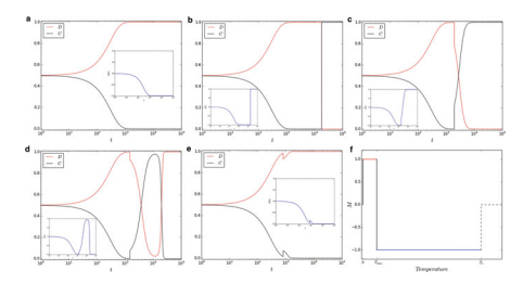
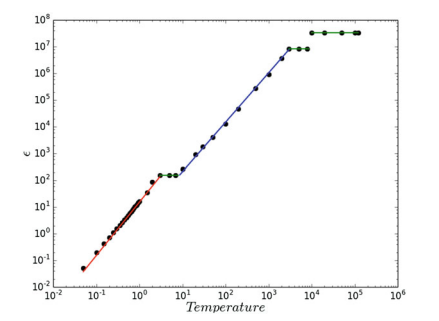
Figure $3.1$ shows the evolution of $G^{b}$, for $\epsilon=1$ on varying $T_{s}$ and, depicted in the inner insets, the variation of system magnetization over time (always inside $G^{b}$ ). As discussed before, in the physical domain of particles, heating the system entails to increase the average speed of particles. Thus, under the assumption that two agents play together if they remain in the same group for a long enough time, we hypothesize that there exists a maximum allowed speed for observing interactions in the form of game (i.e., if the speed is higher than this limit, agents are not able to play the game). This hypothesis requires a critical temperature $T_{c}$, above which no “effective” interactions, in the “information” domain, are possible. As shown in plot (f) of Fig. 3.1, for temperatures in the range $0T_{c}$, a disordered phase emerges at equilibrium. Thus, results of this model suggest that it is always possible to compute a range of temperatures to obtain an equilibrium of full cooperationsee Fig. 3.2. Furthermore, we study the variation of $T_{\max }$ on varying $\epsilon$ (see Fig. 3.3) showing that, even for low $\epsilon$, it is possible to obtain a time $t_{c}$ that allows the system to become cooperative. Eventually, we investigate the relation between the maximum value of $T_{s}$ that allows a population to become cooperative and its size $N$ (i.e., the amount of agents). As shown in Fig. 3.4, the maximum $T_{s}$ scales with $N$ following a power-law function characterized by a scaling parameter $\gamma \sim 2$. The value of $\gamma$ has been computed by considering values of $T_{s}$ shown in Fig. $3.2$ for the case $\epsilon=2$. Finally, it is worth to highlight that all analytical results let emerge a link between the system temperature and its final equilibrium. Recalling that we are not considering the equilibrium of the gas, i.e., it does not thermalize in the proposed model, we emphasize that the equilibrium is considered only in the “information domain.”
计算复杂度理论代考
数学代写|计算复杂度理论代写Computational complexity theory代考|Mean Field Approach
让我们考虑一个由以下人员组成的混合人口ñ代理人,具有初始统一的策略分布(即合作和背叛)。作为条件,所有代理都可以交互,因此,在每个时间步,合作者和背叛者获得的收益可以计算如下:
$$
\left{
圆周率C=(ρC+ñ−1)+(ρd+ñ)小号 圆周率d=(ρC−ñ)吨\正确的。
$$
与ρC+ρd=1,ρC合作者的密度和ρd叛逃者的密度。我们记得,在 PD 中,背叛是主导策略,甚至设置小号=0和
吨=1,它对应于最终平衡,因为圆周率d总是大于圆周率C. 我们记得,通常这些调查是通过使用“无记忆”代理(即,代理无法随着时间的推移累积收益)来执行的,这些代理的交互只与他们的邻居定义,并且一次只关注一个代理(及其对手)。这些条件强烈影响人口的动态。例如,如果我们在每个时间步随机选择一个仅与其邻居交互的代理,原则上可能会发生一系列随机选择连续选择多个密切合作者;因此,在这种情况下,我们可以观察到非常丰富的合作者的出现,即使没有引入像运动这样的机制,也能够战胜叛逃者。此外,当磷=0,同质的叛逃者群体不会增加其整体收益。相反,根据矩阵(3.1),合作群体随着时间的推移不断增加其收益。
现在,我们考虑一个人口被一堵墙分成两组:一组G一个由合作者和混合小组组成Gb(即由合作者和叛逃者组成)。代理只与同一组的成员交互,然后与该组的成员交互G一个永远不会改变,因此,随着时间的推移,它的收益会大大增加。相反的情况发生在群体中Gb,当它收敛到一个有序的背叛阶段时,一旦合作者消失,它的最终回报就会受到限制。在这种情况下,我们可以引入一种策略来修改两组的平衡。特别是,我们可以转向合作,平衡Gb, 并背叛G一个. 在第一种情况下,我们必须等待一段时间,然后将一个或几个合作者移动到Gb, 使叛逃者增加他们的收益,但在修订阶段,他们成为合作者,因为新来者比他们更富有。在第二种情况下,如果我们在几个时间步之后移动一小群叛逃者,Gb至G一个,后者收敛到最终的背叛阶段。这些初步的和理论上的观察让“记忆感知”PD的一个重要特性浮出水面:考虑到两个不同的群体,合作者在长时间单独行动后可能会成功。相反,叛逃者可以通过快速的集体行动获胜。值得注意的是,富有的合作者必须单独行动;否则,他们中的许多人冒着养活叛逃者的风险,即增加太多的回报,从而避免他们改变策略。背叛者则相反,他们集体行动可能会大大降低合作者社区的回报(对于小号<0 ).
数学代写|计算复杂度理论代写Computational complexity theory代考|Mapping Agents to Gas Particles
我们假设可以通过气体动力学理论的框架成功地研究具有移动剂的 PD。因此,这个想法是将代理映射到气体粒子。在这样做时,粒子的平均速度可以计算为⟨在⟩=3吨sķp米p, 和吨s系统温度,ķb玻尔兹曼常数,和米p粒子质量。颗粒被可渗透的壁分成两组。因此,后者可以交叉,但同时避免了停留在相对侧(即,属于不同组)的粒子之间的相互作用。这样做,我们可以对我们的系统提供双重描述:一个在粒子的“物理”域中
另一个在代理的“信息”域中。值得注意的是,为了分析“信息”域中的系统,策略被映射到自旋。总而言之,我们将代理映射到气体粒子以表示其“物理”属性(即随机运动),并将代理使用的策略映射到自旋以表示其“信息”属性(即策略)。这两个映射可以被视为两个不同的层,用于研究代理群体如何随时间演变。尽管物理性质(即运动)会影响代理策略(即其自旋),但可以在两个层/域中独立地达到平衡。最后的观察非常重要,因为我们只对评估“信息”域中达到的最终平衡感兴趣。然后,如前所述,Gb可以用以下等式来描述:
$$
\left{
dρCb(吨)d吨=pCb(吨)⋅ρCb(吨)⋅ρdb(吨)−pdb(吨)⋅ρdb(吨)⋅ρCb(吨) dρdb(吨)d吨=pdb(吨)⋅ρdb(吨)⋅ρCb(吨)−pCb(吨)⋅ρCb(吨)⋅ρdb(吨) ρCb(吨)+ρdb(吨)=1\正确的。
在一世吨H$pCb(吨)$pr○b一个b一世l一世吨是吨H一个吨C○○p和r一个吨○rspr和在一个一世l○nd和F和C吨○rs(一个吨吨一世米和$吨)$一个nd$pdb(吨)$pr○b一个b一世l一世吨是吨H一个吨d和F和C吨○rspr和在一个一世l○nC○○p和r一个吨○rs(一个吨吨一世米和$吨$).吨H和s和pr○b一个b一世l一世吨一世和s一个r和C○米p在吨和d一个CC○rd一世nG吨○吨H和p一个是○FFs○b吨一个一世n和d,一个吨和一个CH吨一世米和s吨和p,b是C○○p和r一个吨○rs一个ndd和F和C吨○rs:
\剩下{
pCb(吨)=圆周率Cb(吨)圆周率Cb(吨)+圆周率db(吨) pdb(吨)=1−pCb(吨)\正确的。
小号是s吨和米(3.3)C一个nb和一个n一个l是吨一世C一个ll是s○l在和dpr○在一世d和d吨H一个吨,一个吨和一个CH吨一世米和s吨和p,在一个l在和s○F$pCb(吨)$一个nd$pdb(吨)$b和在pd一个吨和d.一个CC○rd一世nGl是,吨H和d和ns一世吨是○FC○○p和r一个吨○rsr和一个ds
\rho_{c}^{b}(t)=\frac{\rho_{c}^{b}(0)}{\rho_{c}^{b}(0)-\left[\left(\ rho_{c}^{b}(0)-1\right) \cdot e^{\frac{\pi}{N^{*}}}\right]}
$$
与ρCb(0)合作者的初始密度Gb,τ=pdb(吨)−pCb(吨), 和ñb代理人数Gb. 我们记得那个设置吨s=0,在热力学系统中不允许,对应于静止的情况,导致纳什平衡Gb. 相反,对于吨s>0,我们可以找到更多有趣的场景。现在我们假设,在时间吨=0, 粒子G一个比那些更靠近墙壁Gb(稍后我们将放宽这个约束);例如,让我们考虑一个粒子G一个在其随机路径中,遵循一条长度的轨迹d(在里面n维物理空间)朝向墙壁。假设这个粒子的运动速度等于⟨在⟩, 我们
可以计算穿越的瞬间吨C=d⟨在⟩,即它从G一个至Gb. 因此,在改变温度吨s, 我们可以改变吨C.
观察这两组,我们观察到每个合作者在G一个收益
圆周率C一个=(ρC一个⋅ñ一个−1)⋅吨
而合作者在Gb,根据纳什均衡,随着时间的推移迅速减小。关注收益的变化,最后一个合作者幸存下来Gb, 我们有
$$
\pi_{c}^{b}=\sum_{i=0}^{t}\left[\left(\rho_{c}^{b} \cdot N^{b}-1 \right)+\left(\rho_{d}^{b} \cdot N^{b}\right) S\right] {i} $$ 此外,$\pi {c}^{b} \rightarrow 0一个s\rho_{c}^{b} \rightarrow 0.一个吨t=t_{c},一个n和在C○○p和r一个吨○rr和一个CH和sG^{b}$,收益用公式计算。(3.6)。
数学代写|计算复杂度理论代写Computational complexity theory代考|Result
解析解 (3.5) 允许分析系统的演化并评估初始条件如何影响所提出模型的结果。值得注意的是,如果圆周率C一个(吨C)是“足够大”,新的合作者可能会改变平衡Gb,把叛逃者变成合作者。值得注意的是,考虑计算的收益pCb, 后吨C, 对应于圆周率C一个(吨C), 因为新人是最富有的合作者Gb. 此外,我们注意到圆周率C一个(吨C)取决于ñ一个; 因此,我们通过改变参数来分析系统的演化ε=ñ一个吨ñb,即两组粒子之间的比率。最后,为了数值方便,我们设置ķb=1⋅10−8,米p=1, 和d=1.
数字3.1显示了进化Gb, 为了ε=1在不同的吨s并且,在内部插图中描绘了系统磁化随时间的变化(总是在内部Gb)。如前所述,在粒子的物理域中,加热系统需要增加粒子的平均速度。因此,假设如果两个智能体在同一组中停留足够长的时间,他们会一起玩,我们假设存在一个最大允许的速度以观察游戏形式的交互(即,如果速度高于这个限制,代理不能玩游戏)。这个假设需要一个临界温度吨C,在此之上,在“信息”域中没有“有效”交互是可能的。如图 3.1 的曲线 (f) 所示,对于范围内的温度0吨C,在平衡时出现无序相。因此,该模型的结果表明,总是可以计算一个温度范围以获得完全合作的平衡,见图 3.2。此外,我们研究了吨最大限度在不同的ε(见图 3.3)表明,即使对于低ε, 可以获得时间吨C这允许系统变得合作。最后,我们研究最大值之间的关系吨s允许一个人口变得合作和它的规模ñ(即代理量)。如图 3.4 所示,最大吨s秤与ñ遵循以缩放参数为特征的幂律函数C∼2. 的价值C已通过考虑值计算吨s如图所示。3.2对于这种情况ε=2. 最后,值得强调的是,所有分析结果都让系统温度与其最终平衡之间产生了联系。回想一下我们没有考虑气体的平衡,即在所提出的模型中它没有热化,我们强调仅在“信息域”中考虑平衡。

统计代写请认准statistics-lab™. statistics-lab™为您的留学生涯保驾护航。
金融工程代写
金融工程是使用数学技术来解决金融问题。金融工程使用计算机科学、统计学、经济学和应用数学领域的工具和知识来解决当前的金融问题,以及设计新的和创新的金融产品。
非参数统计代写
非参数统计指的是一种统计方法,其中不假设数据来自于由少数参数决定的规定模型;这种模型的例子包括正态分布模型和线性回归模型。
广义线性模型代考
广义线性模型(GLM)归属统计学领域,是一种应用灵活的线性回归模型。该模型允许因变量的偏差分布有除了正态分布之外的其它分布。
术语 广义线性模型(GLM)通常是指给定连续和/或分类预测因素的连续响应变量的常规线性回归模型。它包括多元线性回归,以及方差分析和方差分析(仅含固定效应)。
有限元方法代写
有限元方法(FEM)是一种流行的方法,用于数值解决工程和数学建模中出现的微分方程。典型的问题领域包括结构分析、传热、流体流动、质量运输和电磁势等传统领域。
有限元是一种通用的数值方法,用于解决两个或三个空间变量的偏微分方程(即一些边界值问题)。为了解决一个问题,有限元将一个大系统细分为更小、更简单的部分,称为有限元。这是通过在空间维度上的特定空间离散化来实现的,它是通过构建对象的网格来实现的:用于求解的数值域,它有有限数量的点。边界值问题的有限元方法表述最终导致一个代数方程组。该方法在域上对未知函数进行逼近。[1] 然后将模拟这些有限元的简单方程组合成一个更大的方程系统,以模拟整个问题。然后,有限元通过变化微积分使相关的误差函数最小化来逼近一个解决方案。
tatistics-lab作为专业的留学生服务机构,多年来已为美国、英国、加拿大、澳洲等留学热门地的学生提供专业的学术服务,包括但不限于Essay代写,Assignment代写,Dissertation代写,Report代写,小组作业代写,Proposal代写,Paper代写,Presentation代写,计算机作业代写,论文修改和润色,网课代做,exam代考等等。写作范围涵盖高中,本科,研究生等海外留学全阶段,辐射金融,经济学,会计学,审计学,管理学等全球99%专业科目。写作团队既有专业英语母语作者,也有海外名校硕博留学生,每位写作老师都拥有过硬的语言能力,专业的学科背景和学术写作经验。我们承诺100%原创,100%专业,100%准时,100%满意。
随机分析代写
随机微积分是数学的一个分支,对随机过程进行操作。它允许为随机过程的积分定义一个关于随机过程的一致的积分理论。这个领域是由日本数学家伊藤清在第二次世界大战期间创建并开始的。
时间序列分析代写
随机过程,是依赖于参数的一组随机变量的全体,参数通常是时间。 随机变量是随机现象的数量表现,其时间序列是一组按照时间发生先后顺序进行排列的数据点序列。通常一组时间序列的时间间隔为一恒定值(如1秒,5分钟,12小时,7天,1年),因此时间序列可以作为离散时间数据进行分析处理。研究时间序列数据的意义在于现实中,往往需要研究某个事物其随时间发展变化的规律。这就需要通过研究该事物过去发展的历史记录,以得到其自身发展的规律。
回归分析代写
多元回归分析渐进(Multiple Regression Analysis Asymptotics)属于计量经济学领域,主要是一种数学上的统计分析方法,可以分析复杂情况下各影响因素的数学关系,在自然科学、社会和经济学等多个领域内应用广泛。
MATLAB代写
MATLAB 是一种用于技术计算的高性能语言。它将计算、可视化和编程集成在一个易于使用的环境中,其中问题和解决方案以熟悉的数学符号表示。典型用途包括:数学和计算算法开发建模、仿真和原型制作数据分析、探索和可视化科学和工程图形应用程序开发,包括图形用户界面构建MATLAB 是一个交互式系统,其基本数据元素是一个不需要维度的数组。这使您可以解决许多技术计算问题,尤其是那些具有矩阵和向量公式的问题,而只需用 C 或 Fortran 等标量非交互式语言编写程序所需的时间的一小部分。MATLAB 名称代表矩阵实验室。MATLAB 最初的编写目的是提供对由 LINPACK 和 EISPACK 项目开发的矩阵软件的轻松访问,这两个项目共同代表了矩阵计算软件的最新技术。MATLAB 经过多年的发展,得到了许多用户的投入。在大学环境中,它是数学、工程和科学入门和高级课程的标准教学工具。在工业领域,MATLAB 是高效研究、开发和分析的首选工具。MATLAB 具有一系列称为工具箱的特定于应用程序的解决方案。对于大多数 MATLAB 用户来说非常重要,工具箱允许您学习和应用专业技术。工具箱是 MATLAB 函数(M 文件)的综合集合,可扩展 MATLAB 环境以解决特定类别的问题。可用工具箱的领域包括信号处理、控制系统、神经网络、模糊逻辑、小波、仿真等。