如果你也在 怎样代写计算复杂度理论Computational complexity theory这个学科遇到相关的难题,请随时右上角联系我们的24/7代写客服。
计算复杂度理论的重点是根据资源使用情况对计算问题进行分类,并将这些类别相互联系起来。计算问题是一项由计算机解决的任务。一个计算问题是可以通过机械地应用数学步骤来解决的,比如一个算法。
statistics-lab™ 为您的留学生涯保驾护航 在代写计算复杂度理论Computational complexity theory方面已经树立了自己的口碑, 保证靠谱, 高质且原创的统计Statistics代写服务。我们的专家在代写计算复杂度理论Computational complexity theory代写方面经验极为丰富,各种代写计算复杂度理论Computational complexity theory相关的作业也就用不着说。
我们提供的计算复杂度理论Computational complexity theory及其相关学科的代写,服务范围广, 其中包括但不限于:
- Statistical Inference 统计推断
- Statistical Computing 统计计算
- Advanced Probability Theory 高等概率论
- Advanced Mathematical Statistics 高等数理统计学
- (Generalized) Linear Models 广义线性模型
- Statistical Machine Learning 统计机器学习
- Longitudinal Data Analysis 纵向数据分析
- Foundations of Data Science 数据科学基础
数学代写|计算复杂度理论代写Computational complexity theory代考|Cook’s Theorem
The notion of reducibilities was first developed in recursion theory. In general, a reducibility $\leq_{r}$ is a binary relation on languages that satisfies the reflexivity and transitivity properties and, hence, it defines a partial ordering on the class of all languages. In this section, we introduce the notion of polynomial-time many-one reducibility. Let $A \subseteq \Sigma^{}$ and $B \subseteq \Gamma^{}$ be two languages. We say that $A$ is many-one reducible to $B$, denoted by $A \leq_{m} B$, if there exists a computable function $f: \Sigma^{} \rightarrow \Gamma^{}$ such that for each $x \in \Sigma^{*}, x \in A$ if and only if $f(x) \in B$. If the reduction function $f$ is further known to be computable in polynomial time, then we say that $A$ is polynomial-time many-one reducible to $B$ and write $A \leq_{m}^{P} B$. It is easy to see that polynomial-time many-one reducibility does satisfy the reflexivity and transitivity properties and, hence, indeed is a reducibility.
Proposition $2.8$ The following hold for all sets $A, B$, and $C$ :
(a) $A \leq_{m}^{P} A$
(b) $A \leq_{m}^{P} B, B \leq_{m}^{P} C \Rightarrow A \leq_{m}^{P} C$.
Note that if $A \leq_{m}^{P} B$ and $B \in P$, then $A \in P$. In general, we say a complexity class $\mathcal{C}$ is closed under the reducibility $\leq_{r}$ if $A \leq_{r} B$ and $B \in \mathcal{C}$ imply $A \in \mathcal{C}$
Proposition 2.9 The complexity classes $P, N P$, and PSPACE are all closed under $\leq_{m}^{P}$
Note that the complexity class $E X P=\bigcup_{c>0} D T I M E\left(2^{c n}\right)$ is not closed under $\leq_{m}^{P}$. People sometimes, therefore, study a weaker class of exponential-time computable sets EXPPOLY = $\bigcup_{k>0} D T I M E\left(2^{n^{k}}\right)$, which is closed under $\leq_{m}^{P}$.
For any complexity class $\mathcal{C}$ that is closed under a reducibility $\leq_{r}$, we say a set $B$ is $\leq_{r}$ hard for class $C$ if $A \leq_{r} B$ for all $A \in \mathcal{C}$ and we say a set $B$ is $\leq_{r}-$ complete for class $\mathcal{C}$ if $B \in \mathcal{C}$ and $B$ is $\leq_{r}$-hard for $\mathcal{C}$. For convenience, we say a set $B$ is $\mathcal{C}$-complete if $B$ is $\leq_{m}^{P}$-complete for the class $\mathcal{C}$. $^{2}$ Thus, a set $B$ is $N P$-complete if $B \in N P$ and $A \leq_{m}^{P} B$ for all $A \in N P$. An $N P$-complete set $B$ is a maximal element in $N P$ under the partial ordering $\leq_{m}^{P}$. Thus, it is not in $P$ if and only if $P \neq N P$.
数学代写|计算复杂度理论代写Computational complexity theory代考|More NP-Complete Problems
The importance of the notion of $N P$-completeness is witnessed by thousands of $N P$-complete problems from a variety of areas in computer science, discrete mathematics, and operations research. Theoretically, all these problems can be proved to be $N P$-complete by reducing SAT to them. It is practically much easier to prove new $N P$-complete problems from some other known $N P$-complete problems that have similar structures as the new problems. In this section, we study some best-known $N P$-complete problems that may be useful to obtain new $N P$-completeness results.
VERTEX COVER (VC): Given a graph $G=(V, E)$ and an integer $K \geq 0$, determine whether $G$ has a vertex cover of size at most $K$, that is, determine whether $V$ has a subset $V^{\prime}$ of size $\leq K$ such that each $e \in E$ has at least one end point in $V^{\prime}$.
Theorem 2.14 VC is NP-complete.
Proof. It is easy to see that $\mathrm{VC}$ is in $N P$. To show that $\mathrm{VC}$ is complete for $N P$, we reduce 3-SAT to it.
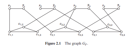
Let $F$ be a 3-CNF formula with $m$ clauses $C_{1}, C_{2}, \ldots, C_{m}$ over $n$ variables $x_{1}, x_{2}, \ldots, x_{n}$. We construct a graph $G_{F}$ of $2 n+3 m$ vertices as follows. The vertices are named $x_{i}, \bar{x}{i}$ for $1 \leq i \leq n$, and $c{j k}$ for $1 \leq j \leq m$, $1 \leq k \leq 3$. The vertices are connected by the following edges: for each $i, 1 \leq i \leq n$, there is an edge connecting $x_{i}$ and $\bar{x}{i}$; for each $j, 1 \leq j \leq m$, there are three edges connecting $c{j, 1}, c_{j, 2}, c_{j, 3}$ into a triangle and, in addition, if $C_{j}=\ell_{1}+\ell_{2}+\ell_{3}$, then there are three edges connecting each $c_{j, k}$ to the vertex named $\ell_{k}, 1 \leq k \leq 3$. Figure $2.1$ shows the graph $G_{F}$ for $F=\left(x_{1}+\bar{x}{2}+x{3}\right)\left(\bar{x}{1}+x{3}+\bar{x}{4}\right)\left(\bar{x}{2}+\bar{x}{3}+x{4}\right) .$
We claim that $F$ is satisfiable if and only if $G_{F}$ has a vertex cover of size $n+2 m$. First, suppose that $F$ is satisfiable by a truth assignment $\tau$. Let $S_{1}=\left{x_{i}: \tau\left(x_{i}\right)=1,1 \leq i \leq n\right} \cup\left{\bar{x}{i}: \tau\left(x{i}\right)=0,1 \leq i \leq n\right}$. Next for each $j, 1 \leq j \leq m$, let $c_{j, j}$ be the vertex of the least index $j_{k}$ such that $c_{j, j_{k}}$ is adjacent to a vertex in $S_{1}$. (By the assumption that $\tau$ satisfies $F$, such an index $j_{k}$ always exists.) Then, let $S_{2}=\left{c_{j, r}: 1 \leq r \leq 3, r \neq j_{k}, 1 \leq j \leq\right.$ $m}$ and $S=S_{1} \cup S_{2}$. It is clear that $S$ is a vertex cover for $G_{F}$ of size $n+2 m$
Conversely, suppose that $G_{F}$ has a vertex cover $S$ of size at most $n+$ $2 m$. As each triangle over $c_{j_{1}}, c_{j_{2}}, c_{j_{3}}$ must have at least two vertices in $S$ and each edge $\left{x_{i}, \bar{x}{i}\right}$ has at least one vertex in $S, S$ is of size exactly $n+2 m$ with exactly two vertices from each triangle $c{j_{1}}, c_{j_{2}}, c_{j_{3}}$ and exactly one vertex from each edge $\left{x_{i}, \bar{x}{i}\right}$. Define $\tau\left(x{i}\right)=1$ if $x_{i} \in S$ and $\tau\left(x_{i}\right)=0$ if $\bar{x}{i} \in S$. Then, each clause $C{j}$ must have a true literal which is the one adjacent to the vertex $c_{j, k}$ that is not in $S$. Thus, $F$ is satisfied by $\tau$.
The above construction is clearly polynomial-time computable. Hence, we have proved 3-SAT $\leq_{m}^{P} V$ VC.
数学代写|计算复杂度理论代写Computational complexity theory代考|Polynomial-Time Turing Reducibility
Polynomial-time many-one reducibility is a strong type of reducibility on decision problems (i.e., languages) that preserves the membership in the class $P$. In this section, we extend this notion to a weaker type of reducibility called polynomial-time Turing reducibility that also preserves the membership in $P$. Moreover, this weak reducibility can also be applied to search problems (i.e., functions).
Intuitively, a problem $A$ is Turing reducible to a problem $B$, denoted by $A \leq_{T} B$, if there is an algorithm $M$ for $A$ which can ask, during its computation, some membership questions about set $B$. If the total amount of time used by $M$ on an input $x$, excluding the querying time, is bounded by $p(|x|)$ for some polynomial $p$, and furthermore, if the length of each query asked by $M$ on input $x$ is also bounded by $p(|x|)$, then we say $A$ is polynomial-time Turing reducible to $B$ and denote it by $A \leq_{T}^{P} B$. Let us look at some examples.
Example $2.20$ (a) For any set $A, \bar{A} \leq_{T}^{P} A$, where $\bar{A}$ is the complement of $A$. This is achieved easily by asking the oracle $A$ whether the input $x$ is in $A$ or not and then reversing the answer. Note that if $N P \neq \operatorname{coNP}$, then $\overline{\mathrm{SAT}}$ is not polynomial-time many-one reducible to SAT. So, this demonstrates that the $\leq_{T}^{P}$-reducibility is potentially weaker than the $\leq_{m}^{P}$-reducibility (cf. Exercise $2.14$ ).
(b) Recall the $N P$-complete problem CLIQUE. We define a variation of the problem CLIQUE as follows:
EXACT-CLIQUE: Given a graph $G=(V, E)$ and an integer $K \geq$ 0 , determine whether it is true that the maximum-size clique of $G$ is of size $K$.
It is not clear whether EXACT-CLIQUE is in $N P$. We can guess a subset $V^{\prime}$ of $V$ of size $K$ and verify in polynomial time that the subgraph of $G$ induced by $V^{\prime}$ is a clique. However, there does not seem to be a nondeterministic algorithm that can check that there is no clique of size greater than $K$ in polynomial time. Therefore, this problem may seem even harder
than the $N P$-complete problem CLIQUE. In the following, however, we show that this problem is actually polynomial-time equivalent to CLIQUE in the sense that they are polynomial-time Turing reducible to each other. Thus, either they are both in $P$ or they are both not in $P$.
First, let us describe an algorithm for the problem CLIQUE that can ask queries to the problem EXACT-CLIQUE. Assume that $G=(V, E)$ is a graph and $K$ is a given integer. We want to know whether there is a clique in $G$ that is of size $K$. We ask whether $(G, k)$ is in EXACT-CLIQUE for each $k=1,2, \ldots,|V|$. Then, we will get the maximum size $k^{}$ of the cliques of $G$. We answer YES to the original problem CLIQUE if and only if $K \leq k^{}$.
Conversely, let $G=(V, E)$ be a graph and $K$ a given integer. Note that the maximum clique size of $G$ is $K$ if and only if $(G, K) \in$ CLIQUE and $(G, K+1) \notin$ CLIQUE. Thus, the question of whether $(G, K) \in$ ExACTCLIQUE can be solved by asking two queries to the problem CLIQUE. (See Exercise 3.3(b) for more studies on EXACT-CLIQUE.)
计算复杂度理论代考
数学代写|计算复杂度理论代写Computational complexity theory代考|Cook’s Theorem
可约性的概念最初是在递归理论中发展起来的。一般来说,可还原性≤r是满足自反性和传递性属性的语言的二元关系,因此,它定义了所有语言类的偏序。在本节中,我们介绍多项式时间多一可约性的概念。让一个⊆Σ和乙⊆Γ是两种语言。我们说一个是多一可归约为乙,表示为一个≤米乙, 如果存在可计算函数F:Σ→Γ这样对于每个X∈Σ∗,X∈一个当且仅当F(X)∈乙. 如果归约函数F进一步知道在多项式时间内是可计算的,那么我们说一个是多项式时间多一可简化为乙和写一个≤米磷乙. 很容易看出,多项式时间多一可约性确实满足自反性和传递性性质,因此确实是可约性。
主张2.8以下适用于所有集合一个,乙, 和C:(
一)一个≤米磷一个
(二)一个≤米磷乙,乙≤米磷C⇒一个≤米磷C.
请注意,如果一个≤米磷乙和乙∈磷, 然后一个∈磷. 一般来说,我们说复杂度类C在可约性下是封闭的≤r如果一个≤r乙和乙∈C意味着一个∈C
命题 2.9 复杂性类磷,ñ磷, 和 PSPACE 都在下关闭≤米磷
注意复杂度类和X磷=⋃C>0D吨我米和(2Cn)不关闭≤米磷. 因此,人们有时会研究较弱的指数时间可计算集 EXPPOLY =⋃ķ>0D吨我米和(2nķ), 下封闭≤米磷.
对于任何复杂度等级C在可还原性下闭合≤r,我们说一个集合乙是≤r很难上课C如果一个≤r乙对所有人一个∈C我们说一组乙是≤r−完成上课C如果乙∈C和乙是≤r-很难C. 为方便起见,我们称一组乙是C-完成如果乙是≤米磷- 完成课程C. 2于是,一组乙是ñ磷-完成如果乙∈ñ磷和一个≤米磷乙对所有人一个∈ñ磷. 一个ñ磷-全套乙是最大元素ñ磷在偏序下≤米磷. 因此,它不在磷当且仅当磷≠ñ磷.
数学代写|计算复杂度理论代写Computational complexity theory代考|More NP-Complete Problems
概念的重要性ñ磷- 完整性被成千上万的人见证ñ磷- 完成计算机科学、离散数学和运筹学各个领域的问题。理论上,所有这些问题都可以证明是ñ磷-通过减少SAT来完成。证明新的实际上要容易得多ñ磷- 来自其他一些已知问题的完整问题ñ磷- 完成与新问题具有相似结构的问题。在本节中,我们研究了一些最著名的ñ磷-完成可能对获得新的有用的问题ñ磷- 完整性结果。
VERTEX COVER (VC):给定一个图G=(在,和)和一个整数ķ≥0, 判断是否G最多有一个 size 的顶点覆盖ķ,即判断是否在有一个子集在′大小的≤ķ使得每个和∈和至少有一个端点在在′.
定理 2.14 VC 是 NP 完全的。
证明。很容易看出在C在ñ磷. 为了表明在C是完整的ñ磷,我们将 3-SAT 减少到它。
让F是一个 3-CNF 公式米条款C1,C2,…,C米超过n变量X1,X2,…,Xn. 我们构建一个图GF的2n+3米顶点如下。顶点被命名X一世,X¯一世为了1≤一世≤n, 和Cjķ为了1≤j≤米, 1≤ķ≤3. 顶点由以下边连接:对于每个一世,1≤一世≤n, 有一条边连接X一世和X¯一世; 对于每个j,1≤j≤米, 有三个边连接Cj,1,Cj,2,Cj,3成一个三角形,此外,如果Cj=ℓ1+ℓ2+ℓ3,则有三个边连接每个Cj,ķ到名为的顶点ℓķ,1≤ķ≤3. 数字2.1显示图表GF为了F=(X1+X¯2+X3)(X¯1+X3+X¯4)(X¯2+X¯3+X4).
我们声称F是可满足的当且仅当GF有一个大小为的顶点覆盖n+2米. 首先,假设F可以通过真值分配来满足τ. 让S_{1}=\left{x_{i}: \tau\left(x_{i}\right)=1,1 \leq i \leq n\right} \cup\left{\bar{x}{i }: \tau\left(x{i}\right)=0,1 \leq i \leq n\right}S_{1}=\left{x_{i}: \tau\left(x_{i}\right)=1,1 \leq i \leq n\right} \cup\left{\bar{x}{i }: \tau\left(x{i}\right)=0,1 \leq i \leq n\right}. 接下来为每个j,1≤j≤米, 让Cj,j是最小索引的顶点jķ这样Cj,jķ与中的一个顶点相邻小号1. (假设τ满足F, 这样的索引jķ总是存在的。)然后,让S_{2}=\left{c_{j, r}: 1 \leq r \leq 3, r \neq j_{k}, 1 \leq j \leq\right.$ $m}S_{2}=\left{c_{j, r}: 1 \leq r \leq 3, r \neq j_{k}, 1 \leq j \leq\right.$ $m}和小号=小号1∪小号2. 很清楚小号是一个顶点覆盖GF大小的n+2米
相反,假设GF有一个顶点覆盖小号最多大小n+ 2米. 当每个三角形超过Cj1,Cj2,Cj3必须至少有两个顶点小号和每条边\left{x_{i}, \bar{x}{i}\right}\left{x_{i}, \bar{x}{i}\right}至少有一个顶点在小号,小号大小正好n+2米每个三角形恰好有两个顶点Cj1,Cj2,Cj3并且每条边恰好有一个顶点\left{x_{i}, \bar{x}{i}\right}\left{x_{i}, \bar{x}{i}\right}. 定义τ(X一世)=1如果X一世∈小号和τ(X一世)=0如果X¯一世∈小号. 然后,每个子句Cj必须有一个真正的文字,它是与顶点相邻的文字Cj,ķ那不在小号. 因此,F满足于τ.
上述结构显然是多项式时间可计算的。因此,我们证明了 3-SAT≤米磷在风险投资。
数学代写|计算复杂度理论代写Computational complexity theory代考|Polynomial-Time Turing Reducibility
多项式时间多一可约性是决策问题(即语言)的一种强可约性类型,它保留了类中的成员资格磷. 在本节中,我们将这个概念扩展到一种较弱的可约性类型,称为多项式时间图灵可约性,它也保留了磷. 此外,这种弱可约性也可以应用于搜索问题(即函数)。
直觉上是个问题一个图灵是否可以简化为一个问题乙,表示为一个≤吨乙, 如果有算法米为了一个它可以在计算过程中询问一些关于集合的成员问题乙. 如果使用的总时间米在输入X,不包括查询时间,有界p(|X|)对于一些多项式p,此外,如果每个查询的长度由米在输入X也受p(|X|),那么我们说一个是多项式时间图灵可简化为乙并表示为一个≤吨磷乙. 让我们看一些例子。
例子2.20(a) 对于任何集合一个,一个¯≤吨磷一个, 在哪里一个¯是的补码一个. 这很容易通过询问神谕来实现一个是否输入X在一个或不,然后颠倒答案。请注意,如果ñ磷≠配比, 然后小号一个吨¯不是多项式时间多一可简化为 SAT。因此,这表明≤吨磷- 可还原性可能比≤米磷-可还原性(参见练习2.14)。
(b) 回顾ñ磷-完成问题CLIQUE。我们将问题 CLIQUE 的一个变体定义如下:
EXACT-CLIQUE:给定一个图G=(在,和)和一个整数ķ≥0 , 判断最大大小的团是否为真G是大小ķ.
尚不清楚 EXACT-CLIQUE 是否在ñ磷. 我们可以猜测一个子集在′的在大小的ķ并在多项式时间内验证G由…介绍在′是一个集团。但是,似乎没有一种非确定性算法可以检查是否存在大小不大于ķ在多项式时间内。因此,这个问题可能看起来更难
比ñ磷-完成问题CLIQUE。然而,在下文中,我们展示了这个问题实际上是多项式时间等价于 CLIQUE,因为它们是多项式时间图灵可相互约简的。因此,要么他们都在磷或者他们都不在磷.
首先,让我们描述一个针对问题 CLIQUE 的算法,该算法可以对问题 EXACT-CLIQUE 进行查询。假使,假设G=(在,和)是一个图并且ķ是一个给定的整数。我们想知道是否有派系G那是大小ķ. 我们问是否(G,ķ)每个都在 EXACT-CLIQUE 中ķ=1,2,…,|在|. 然后,我们将得到最大尺寸ķ的派系G. 当且仅当我们对原始问题 CLIQUE 回答“是”ķ≤ķ.
反之,让G=(在,和)是一个图形和ķ给定的整数。请注意,最大集团规模G是ķ当且仅当(G,ķ)∈集团和(G,ķ+1)∉集团。因此,是否(G,ķ)∈ExACTCLIQUE 可以通过对问题 CLIQUE 进行两次查询来解决。(有关 EXACT-CLIQUE 的更多研究,请参见练习 3.3(b)。)

统计代写请认准statistics-lab™. statistics-lab™为您的留学生涯保驾护航。
金融工程代写
金融工程是使用数学技术来解决金融问题。金融工程使用计算机科学、统计学、经济学和应用数学领域的工具和知识来解决当前的金融问题,以及设计新的和创新的金融产品。
非参数统计代写
非参数统计指的是一种统计方法,其中不假设数据来自于由少数参数决定的规定模型;这种模型的例子包括正态分布模型和线性回归模型。
广义线性模型代考
广义线性模型(GLM)归属统计学领域,是一种应用灵活的线性回归模型。该模型允许因变量的偏差分布有除了正态分布之外的其它分布。
术语 广义线性模型(GLM)通常是指给定连续和/或分类预测因素的连续响应变量的常规线性回归模型。它包括多元线性回归,以及方差分析和方差分析(仅含固定效应)。
有限元方法代写
有限元方法(FEM)是一种流行的方法,用于数值解决工程和数学建模中出现的微分方程。典型的问题领域包括结构分析、传热、流体流动、质量运输和电磁势等传统领域。
有限元是一种通用的数值方法,用于解决两个或三个空间变量的偏微分方程(即一些边界值问题)。为了解决一个问题,有限元将一个大系统细分为更小、更简单的部分,称为有限元。这是通过在空间维度上的特定空间离散化来实现的,它是通过构建对象的网格来实现的:用于求解的数值域,它有有限数量的点。边界值问题的有限元方法表述最终导致一个代数方程组。该方法在域上对未知函数进行逼近。[1] 然后将模拟这些有限元的简单方程组合成一个更大的方程系统,以模拟整个问题。然后,有限元通过变化微积分使相关的误差函数最小化来逼近一个解决方案。
tatistics-lab作为专业的留学生服务机构,多年来已为美国、英国、加拿大、澳洲等留学热门地的学生提供专业的学术服务,包括但不限于Essay代写,Assignment代写,Dissertation代写,Report代写,小组作业代写,Proposal代写,Paper代写,Presentation代写,计算机作业代写,论文修改和润色,网课代做,exam代考等等。写作范围涵盖高中,本科,研究生等海外留学全阶段,辐射金融,经济学,会计学,审计学,管理学等全球99%专业科目。写作团队既有专业英语母语作者,也有海外名校硕博留学生,每位写作老师都拥有过硬的语言能力,专业的学科背景和学术写作经验。我们承诺100%原创,100%专业,100%准时,100%满意。
随机分析代写
随机微积分是数学的一个分支,对随机过程进行操作。它允许为随机过程的积分定义一个关于随机过程的一致的积分理论。这个领域是由日本数学家伊藤清在第二次世界大战期间创建并开始的。
时间序列分析代写
随机过程,是依赖于参数的一组随机变量的全体,参数通常是时间。 随机变量是随机现象的数量表现,其时间序列是一组按照时间发生先后顺序进行排列的数据点序列。通常一组时间序列的时间间隔为一恒定值(如1秒,5分钟,12小时,7天,1年),因此时间序列可以作为离散时间数据进行分析处理。研究时间序列数据的意义在于现实中,往往需要研究某个事物其随时间发展变化的规律。这就需要通过研究该事物过去发展的历史记录,以得到其自身发展的规律。
回归分析代写
多元回归分析渐进(Multiple Regression Analysis Asymptotics)属于计量经济学领域,主要是一种数学上的统计分析方法,可以分析复杂情况下各影响因素的数学关系,在自然科学、社会和经济学等多个领域内应用广泛。
MATLAB代写
MATLAB 是一种用于技术计算的高性能语言。它将计算、可视化和编程集成在一个易于使用的环境中,其中问题和解决方案以熟悉的数学符号表示。典型用途包括:数学和计算算法开发建模、仿真和原型制作数据分析、探索和可视化科学和工程图形应用程序开发,包括图形用户界面构建MATLAB 是一个交互式系统,其基本数据元素是一个不需要维度的数组。这使您可以解决许多技术计算问题,尤其是那些具有矩阵和向量公式的问题,而只需用 C 或 Fortran 等标量非交互式语言编写程序所需的时间的一小部分。MATLAB 名称代表矩阵实验室。MATLAB 最初的编写目的是提供对由 LINPACK 和 EISPACK 项目开发的矩阵软件的轻松访问,这两个项目共同代表了矩阵计算软件的最新技术。MATLAB 经过多年的发展,得到了许多用户的投入。在大学环境中,它是数学、工程和科学入门和高级课程的标准教学工具。在工业领域,MATLAB 是高效研究、开发和分析的首选工具。MATLAB 具有一系列称为工具箱的特定于应用程序的解决方案。对于大多数 MATLAB 用户来说非常重要,工具箱允许您学习和应用专业技术。工具箱是 MATLAB 函数(M 文件)的综合集合,可扩展 MATLAB 环境以解决特定类别的问题。可用工具箱的领域包括信号处理、控制系统、神经网络、模糊逻辑、小波、仿真等。