如果你也在 怎样代写随机过程统计Stochastic process statistics这个学科遇到相关的难题,请随时右上角联系我们的24/7代写客服。
随机过程 用于表示在时间上发展的统计现象以及在处理这些现象时出现的理论模型,由于这些现象在许多领域都会遇到,因此这篇文章具有广泛的实际意义。
statistics-lab™ 为您的留学生涯保驾护航 在代写随机过程统计Stochastic process statistics方面已经树立了自己的口碑, 保证靠谱, 高质且原创的统计Statistics代写服务。我们的专家在代写随机过程统计Stochastic process statistics代写方面经验极为丰富,各种代写随机过程统计Stochastic process statistics相关的作业也就用不着说。
我们提供的随机过程统计Stochastic process statistics及其相关学科的代写,服务范围广, 其中包括但不限于:
- Statistical Inference 统计推断
- Statistical Computing 统计计算
- Advanced Probability Theory 高等概率论
- Advanced Mathematical Statistics 高等数理统计学
- (Generalized) Linear Models 广义线性模型
- Statistical Machine Learning 统计机器学习
- Longitudinal Data Analysis 纵向数据分析
- Foundations of Data Science 数据科学基础
数学代写|随机过程统计代写Stochastic process statistics代考|Optimization with Constraints: Feasible Region
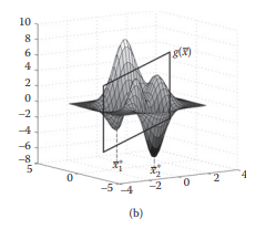
The objective function is the heart of an optimization problem, since it is the function that should be minimized or maximized. When the optimization situation involves only the analysis of the objective function, as shown in Figure 1.3, it is said that the problem is unconstrained, and the search for the solution occurs in the entire set of $R^{n}$. Nevertheless, for most of the practical problems, the variables are not unbounded; thus, the search space is reduced by the introduction of bounds for the variables. Furthermore, most of the variables appearing on the objective function are related to other variables through a mathematical model, which implies that the search space for the objective function is even more reduced. The region in the $n$-dimensional space limited by those bounds for the variables and the equations relating the set of variables is known as the feasible region. In Figure $1.4 a$, a feasible region in a bidimensional space can be observed, which is enclosed by the constraints $h_{1}(x), h_{2}(x)$, and $g_{1}(x)$. On the other hand, Figure $1.4 \mathrm{~b}$ shows a tridimensional feasible region, where the constraint $g(\bar{x})$ is a plane, and the objective function is a surface with various minimums. Until now, two types of constraints have been mentioned, $h(\bar{x})$ and $g(\bar{x})$. The difference between the two types of constraints is explained. The equations $h(\bar{x})$ are equality constraints, i.e., they have the structure $h(\bar{x})=0$. Such constraints should be strictly complied. Thus, they reduce even more the number of feasible solutions. On the other hand, the equations $g(\bar{x})$ are inequality constraints, i.e.,$g(\bar{x}) \leq 0$. Such constraints can be complied as an equality, $g(\bar{x})=0$, for which it is said that the constraint is active; or they can be complied as an inequality, $g(\bar{x})<0$, for which it said that the constraint is inactive. The inequality constraints, thus, are more easily complied, because they allow the feasible region to include higher number of solutions.
数学代写|随机过程统计代写Stochastic process statistics代考|Multiobjective Optimization
At this point, the objective function has been mentioned as a measurement of the goodness of a given solution. It has been stated that an optimization problem, where there is only the necessity of maximizing/minimizing a given objective function, is known as an unconstrained problem. On the other hand, the optimization problem may involve constraints, which limits
the solution space for the objective function. Nevertheless, there are cases on which it is desired to simultaneously optimize two or more objective functions subject to the same set of constraints and variables. This is called multiobjective optimization. This type of problems can be represented in the following general formulation:
optimize $\bar{Z}=\left(Z_{1}, Z_{2}, \ldots, Z_{k}\right)$
s.t.
$h(\bar{x})=0$
$g(\bar{x}) \leq 0$
where $k$ is the total number of objectives, $\bar{Z}$ is the vector of objective functions, and $Z_{1}=z_{1}(\bar{x}), Z_{2}=z_{2}(\bar{x})$, and so on are the individual objective functions. As it is observed, the feasible regions, i.e., the constraints of the optimization problem, are the same for all the objectives. Thus, the only difference with the optimization problem given in Equation $1.8$ is that there are more than one objective functions, and the solution complies with all of them and also with the constraints.
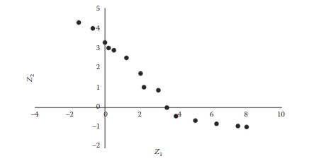
Let us imagine about a problem with two objectives. Both objective functions may have their minimum (or maximum) on the same (or almost on the same) point $\bar{x}$, as shown in Figure $1.5 \mathrm{a}$. Nevertheless, such a problem could even be stated as a problem with a single objective. A more interesting situation occurs when the minimum of the objective functions occur for a different set of $\bar{x}$ values, which implies that when one of the objectives is being reduced, the other one increases (Figure $1.5 \mathrm{~b}$ ). When two objective functions follow such performance, it is mentioned that they are in competence. This implies that, when the minimum for one of the objective functions occurs, the other objective has a value far from its own minimum. Thus, assuming, in general, a situation with $k$ objective functions, the solution to the optimization problem should be a compromise
among all the objectives, since the better solution for one of the objectives could be a considerably inadequate solution for the others. An important concept in multiobjective optimization is the nondominated solution. In mathematical terms, it can be mentioned that $\bar{x}^{}$ is a nondominated solution for a minimization problem if, for any other feasible solution $\bar{x}$, the following relationship is true: $$ Z_{p}(\bar{x}) \leq Z_{p}\left(\bar{x}^{}\right)
$$
数学代写|随机过程统计代写Stochastic process statistics代考|Weighted Sum Method
In this method, the optimization problem shown in Equation $1.9$ is modified as follows:
$$
\begin{aligned}
&\text { optimize } Z_{\text {mult }}=\sum_{i=1}^{k} \omega_{i} Z_{i} \
&\text { s.t. } \
&h(\bar{x})=0 \
&g(\bar{x}) \leq 0
\end{aligned}
$$
Thus, the vector of objectives is substituted by a linear combination of the individual objectives. The parameters $\omega_{i}$ are known as weights. In the weighing method, the function $Z_{\text {mult }}$ is used for generating the Pareto front. In the first approach, $k$ individual optimization problems are solved for each objective function. In other words, the problem is first solved by setting one of the $\omega_{i}^{\prime}$ s as 1 and the other weights as zero, and so on, until the optimal for each individual objective function has been found. Those points represent the extremes at the Pareto front. Then, the intermediate solutions are obtained by testing different combinations of $\omega_{i}$, which provide more or less importance to each $Z_{i}$. Certainly, particular care should be provided on the scale of each objective functions for a proper selection of the values of the weights, in order to have equality on the contributions of each individual objective to $Z_{\text {mult- }}$
随机过程统计代考
数学代写|随机过程统计代写Stochastic process statistics代考|Optimization with Constraints: Feasible Region
目标函数是优化问题的核心,因为它是应该最小化或最大化的函数。当优化情况只涉及目标函数的分析时,如图 1.3 所示,称问题是无约束的,寻找解发生在整个集合中Rn. 然而,对于大多数实际问题来说,变量并不是无界的;因此,通过引入变量边界来减少搜索空间。此外,目标函数上出现的大多数变量都通过数学模型与其他变量相关,这意味着目标函数的搜索空间更加缩小。该地区在n由变量和与变量集相关的方程限制的维空间称为可行区域。如图1.4一个,可以观察到一个二维空间中的可行域,它被约束包围H1(X),H2(X), 和G1(X). 另一方面,图1.4 b显示了一个三维可行域,其中约束G(X¯)是一个平面,目标函数是一个具有各种最小值的曲面。到目前为止,已经提到了两种类型的约束,H(X¯)和G(X¯). 解释了两种类型的约束之间的区别。方程H(X¯)是等式约束,即它们具有结构H(X¯)=0. 应严格遵守此类约束。因此,它们甚至更多地减少了可行解决方案的数量。另一方面,方程G(X¯)是不等式约束,即G(X¯)≤0. 这样的约束可以被遵守为等式,G(X¯)=0, 据说约束是活动的;或者它们可以被遵守为不等式,G(X¯)<0,它说约束是不活动的。因此,不等式约束更容易遵守,因为它们允许可行区域包含更多数量的解决方案。
数学代写|随机过程统计代写Stochastic process statistics代考|Multiobjective Optimization
在这一点上,已经提到目标函数作为给定解决方案的好坏的度量。已经说过,只有最大化/最小化给定目标函数的必要性的优化问题被称为无约束问题。另一方面,优化问题可能涉及约束,这限制了
目标函数的解空间。然而,在某些情况下,希望同时优化两个或多个受同一组约束和变量约束的目标函数。这称为多目标优化。这类问题可以用以下一般公式表示:
优化从¯=(从1,从2,…,从ķ)
英石
H(X¯)=0
G(X¯)≤0
在哪里ķ是目标的总数,从¯是目标函数的向量,并且从1=和1(X¯),从2=和2(X¯), 等等是个体目标函数。正如所观察到的,可行区域,即优化问题的约束,对于所有目标都是相同的。因此,与方程中给出的优化问题的唯一区别1.8是存在不止一个目标函数,并且解决方案符合所有这些目标并且也符合约束条件。
让我们想象一个有两个目标的问题。两个目标函数的最小值(或最大值)可能在相同(或几乎相同)点上X¯,如图1.5一个. 然而,这样的问题甚至可以说是一个单一目标的问题。当目标函数的最小值出现在不同的一组X¯值,这意味着当其中一个目标减少时,另一个目标增加(图1.5 b)。当两个目标函数遵循这样的表现时,就会提到它们是有能力的。这意味着,当一个目标函数的最小值出现时,另一个目标的值远离它自己的最小值。因此,假设,一般情况下,ķ目标函数,优化问题的解决方案应该是一个折衷
在所有目标中,因为其中一个目标的更好解决方案可能是其他目标的一个相当不充分的解决方案。多目标优化中的一个重要概念是非支配解。用数学术语来说,可以提到X¯是最小化问题的非支配解,如果,对于任何其他可行解X¯,以下关系成立:
从p(X¯)≤从p(X¯)
数学代写|随机过程统计代写Stochastic process statistics代考|Weighted Sum Method
在这种方法中,优化问题如方程所示1.9修改如下:
优化 从很多 =∑一世=1ķω一世从一世 英石 H(X¯)=0 G(X¯)≤0
因此,目标向量被各个目标的线性组合所取代。参数ω一世被称为权重。在称重方法中,函数从很多 用于生成帕累托前沿。在第一种方法中,ķ为每个目标函数求解单独的优化问题。换句话说,首先通过设置一个ω一世′s 为 1,其他权重为 0,依此类推,直到找到每个单独目标函数的最优值。这些点代表了帕累托前沿的极端情况。然后,通过测试不同的组合得到中间解ω一世,它们或多或少地对每个从一世. 当然,应特别注意每个目标函数的尺度,以正确选择权重值,以使每个单独目标对从很多-

统计代写请认准statistics-lab™. statistics-lab™为您的留学生涯保驾护航。
金融工程代写
金融工程是使用数学技术来解决金融问题。金融工程使用计算机科学、统计学、经济学和应用数学领域的工具和知识来解决当前的金融问题,以及设计新的和创新的金融产品。
非参数统计代写
非参数统计指的是一种统计方法,其中不假设数据来自于由少数参数决定的规定模型;这种模型的例子包括正态分布模型和线性回归模型。
广义线性模型代考
广义线性模型(GLM)归属统计学领域,是一种应用灵活的线性回归模型。该模型允许因变量的偏差分布有除了正态分布之外的其它分布。
术语 广义线性模型(GLM)通常是指给定连续和/或分类预测因素的连续响应变量的常规线性回归模型。它包括多元线性回归,以及方差分析和方差分析(仅含固定效应)。
有限元方法代写
有限元方法(FEM)是一种流行的方法,用于数值解决工程和数学建模中出现的微分方程。典型的问题领域包括结构分析、传热、流体流动、质量运输和电磁势等传统领域。
有限元是一种通用的数值方法,用于解决两个或三个空间变量的偏微分方程(即一些边界值问题)。为了解决一个问题,有限元将一个大系统细分为更小、更简单的部分,称为有限元。这是通过在空间维度上的特定空间离散化来实现的,它是通过构建对象的网格来实现的:用于求解的数值域,它有有限数量的点。边界值问题的有限元方法表述最终导致一个代数方程组。该方法在域上对未知函数进行逼近。[1] 然后将模拟这些有限元的简单方程组合成一个更大的方程系统,以模拟整个问题。然后,有限元通过变化微积分使相关的误差函数最小化来逼近一个解决方案。
tatistics-lab作为专业的留学生服务机构,多年来已为美国、英国、加拿大、澳洲等留学热门地的学生提供专业的学术服务,包括但不限于Essay代写,Assignment代写,Dissertation代写,Report代写,小组作业代写,Proposal代写,Paper代写,Presentation代写,计算机作业代写,论文修改和润色,网课代做,exam代考等等。写作范围涵盖高中,本科,研究生等海外留学全阶段,辐射金融,经济学,会计学,审计学,管理学等全球99%专业科目。写作团队既有专业英语母语作者,也有海外名校硕博留学生,每位写作老师都拥有过硬的语言能力,专业的学科背景和学术写作经验。我们承诺100%原创,100%专业,100%准时,100%满意。
随机分析代写
随机微积分是数学的一个分支,对随机过程进行操作。它允许为随机过程的积分定义一个关于随机过程的一致的积分理论。这个领域是由日本数学家伊藤清在第二次世界大战期间创建并开始的。
时间序列分析代写
随机过程,是依赖于参数的一组随机变量的全体,参数通常是时间。 随机变量是随机现象的数量表现,其时间序列是一组按照时间发生先后顺序进行排列的数据点序列。通常一组时间序列的时间间隔为一恒定值(如1秒,5分钟,12小时,7天,1年),因此时间序列可以作为离散时间数据进行分析处理。研究时间序列数据的意义在于现实中,往往需要研究某个事物其随时间发展变化的规律。这就需要通过研究该事物过去发展的历史记录,以得到其自身发展的规律。
回归分析代写
多元回归分析渐进(Multiple Regression Analysis Asymptotics)属于计量经济学领域,主要是一种数学上的统计分析方法,可以分析复杂情况下各影响因素的数学关系,在自然科学、社会和经济学等多个领域内应用广泛。
MATLAB代写
MATLAB 是一种用于技术计算的高性能语言。它将计算、可视化和编程集成在一个易于使用的环境中,其中问题和解决方案以熟悉的数学符号表示。典型用途包括:数学和计算算法开发建模、仿真和原型制作数据分析、探索和可视化科学和工程图形应用程序开发,包括图形用户界面构建MATLAB 是一个交互式系统,其基本数据元素是一个不需要维度的数组。这使您可以解决许多技术计算问题,尤其是那些具有矩阵和向量公式的问题,而只需用 C 或 Fortran 等标量非交互式语言编写程序所需的时间的一小部分。MATLAB 名称代表矩阵实验室。MATLAB 最初的编写目的是提供对由 LINPACK 和 EISPACK 项目开发的矩阵软件的轻松访问,这两个项目共同代表了矩阵计算软件的最新技术。MATLAB 经过多年的发展,得到了许多用户的投入。在大学环境中,它是数学、工程和科学入门和高级课程的标准教学工具。在工业领域,MATLAB 是高效研究、开发和分析的首选工具。MATLAB 具有一系列称为工具箱的特定于应用程序的解决方案。对于大多数 MATLAB 用户来说非常重要,工具箱允许您学习和应用专业技术。工具箱是 MATLAB 函数(M 文件)的综合集合,可扩展 MATLAB 环境以解决特定类别的问题。可用工具箱的领域包括信号处理、控制系统、神经网络、模糊逻辑、小波、仿真等。