如果你也在 怎样代写计算复杂性理论computational complexity theory这个学科遇到相关的难题,请随时右上角联系我们的24/7代写客服。
计算复杂性理论computational complexity theory的重点是根据资源使用情况对计算问题进行分类,并将这些类别相互联系起来。计算问题是一项由计算机解决的任务。一个计算问题是可以通过机械地应用数学步骤来解决的,比如一个算法。
statistics-lab™ 为您的留学生涯保驾护航 在代写计算复杂性理论computational complexity theory方面已经树立了自己的口碑, 保证靠谱, 高质且原创的统计Statistics代写服务。我们的专家在代写计算复杂性理论computational complexity theory代写方面经验极为丰富,各种代写计算复杂性理论相关的作业也就用不着说。
我们提供的计算复杂性理论computational complexity theory及其相关学科的代写,服务范围广, 其中包括但不限于:
- Statistical Inference 统计推断
- Statistical Computing 统计计算
- Advanced Probability Theory 高等概率论
- Advanced Mathematical Statistics 高等数理统计学
- (Generalized) Linear Models 广义线性模型
- Statistical Machine Learning 统计机器学习
- Longitudinal Data Analysis 纵向数据分析
- Foundations of Data Science 数据科学基础
数学代考|计算复杂性理论代写computational complexity theory代考|Transient Lengths and Cycle Periods
For any cellular automata acting on a finite state space, every state eventually maps to a fixed point or cycle. If a rule is injective, it is reversible and every state is a fixed point, or is on a cycle. If not injective, there will be states without predecessors, Garden-of-Eden states. As indicate, however, if a rule is additive its Garden-of-Eden states are spurious in the sense that they do have predecessors if the state space is enlarged.
The following theorem lists several significant properties of cellular automata rules acting on $\mathcal{E}(\mathcal{A}, \mathcal{Z})$ or $\mathcal{E}\left(\mathcal{A}, \mathcal{Z}^{+}\right)$with left justified neighborhoods.
Theorem 3 ([81]) Let $\mathcal{X}$ be a $k$-site cellular automata rule acting on $\mathcal{E}(\mathcal{A}, \mathcal{Z})$ or on $\mathcal{E}\left(\mathcal{A}, Z^{+}\right)$with left justified neighborhoods. Then the following statements are equivalent: (a) $X$ is surjective, (b) $\chi$ has an empty Garden-ofEden, (c) Every finite sequence $\mu_{0} \ldots \mu_{n-1}$ has exactly $p^{k-1}$ pre-images and every state $\mu$ has at most $p^{k-1}$ predecessors, (d) $\mathcal{X}$ maps eventually periodic states to eventually periodic states and non-periodic states to non-periodic states, (e) as a map of the interval $[0,1] X$ maps rationals to rationals and irrationals to irrationals.
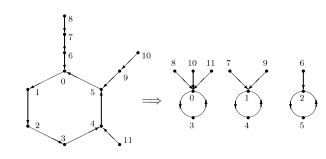
If $\mathcal{X}: \mathcal{E}\left(\mathcal{A}, \mathcal{Z}{n}\right) \mapsto \mathcal{E}\left(\mathcal{A}, \mathcal{Z}{n}\right)$ is a $k$-site rule with $|\mathcal{A}|=p$ and either periodic or null boundary conditions, the state transition diagram, $\operatorname{STD}(\mathcal{X})$ is a graph with $p^{n}$ vertices labeled by the set of $p$-adic numbers $\left{i_{0}, \ldots, i_{n-1} \mid 0 \leq i_{r} \leq p-1\right}$. An edge is directed from the vertex $i_{0}, \ldots, i_{n-1}$ to the vertex $j_{0}, \ldots, j_{n-1}$ if and only if $\chi\left(i_{0}, \ldots, i_{n-1}\right)=j_{0}, \ldots, j_{n-1}$. Each state $\mu$ maps to a unique state $\mathcal{X}(\mu)$ so $\operatorname{STD}(\mathcal{X})$ consists of a set of trees rooted on fixed points or cycles. States at the top of trees are Garden-of-Eden states.
If $h(\mathcal{X}, n)$ is the maximum tree height, states at heights $h \leq h(\mathcal{X}, n)$ cannot appear after $h(\mathcal{X}, n)-h+1$ iterations and after $h(\mathcal{X}, n)$ iterations only fixed points and states on cycles remain. Thus, iteration of a non-injective rule on $\mathcal{E}\left(\mathcal{A}, \mathcal{Z}{n}\right)$ decreases the number of available states with a corresponding reduction in entropy. On the other hand, non-injective additive rules acting on $\mathcal{E}\left(\mathcal{A}, Z^{+}\right)$ do not reduce entropy [117] even though the do so on $\mathcal{E}\left(\mathcal{A}, Z{n}\right)$ for all $n$. The explanation for this apparent paradox is that the Garden-of-Eden states that appear in $\mathcal{E}\left(\mathcal{A}, Z_{n}\right)$ are artifacts of the finite length of states in this space. When embedded in $Z^{+}$, states in $Z_{n}$ correspond to periodic configurations, hence to rational numbers in $[0,1]$ and the set of all rationals has measure 0 in the reals.
Parameters of interest for characterizing state transition diagrams of rules acting on $\mathcal{E}\left(\mathcal{A}, Z_{n}\right)$ are the maximum tree height $h(\mathcal{X}, n)$ and the cycle periods $c_{s}(\mathcal{X}, n)$
数学代考|计算复杂性理论代写computational complexity theory代考|Computing Predecessor States
A problem of general interest for cellular automata is computation of predecessor states. For a rule $\mathcal{X}: \mathbb{E}(\mathcal{A}, \mathcal{L}) \mapsto \mathcal{E}(\mathcal{A}, \mathcal{L})$ with a state $\beta$ given this requires solution of the equation $\mathcal{X}(\mu)=\beta$. It is always possible to construct solutions for this equation, or to show that none exist by a method of backward reconstruction based on the rule table.
Example 7 (Rule 60 Acting on $Z_{4}$ With Periodic Boundary Conditions) Rule 60 is a 2 -site rule, defined by $(00,11) \mapsto 0,(01,10) \mapsto 1$. Given the state 0110 the predecessors of this state can be computed as follows:
- The initial 0 in 0110 can arise from either 00 or 11 .
- Starting with a 00, the next symbol in 0110 is a 1 and this can arise from a 01 or a 10 , but this must also connect to the original 00 so only 01 is allowed, giving 001 . Starting from a 11, on the other hand, the same reasoning requires 110 .
- The third symbol in 0110 is also a 1 . To be consistent with 001 requires that 10 be selected, and to be consistent with 110 requires that 01 be selected, thus giving the two partially constructed possibilities as 0010 and 1101 .
- Finally, the fourth symbol must be a 0 . This requires that the predecessor string conclude with either 00 or 11. Since the strings are in $Z_{4}$ with periodic boundary conditions, the final symbol in the predecessor string must also be the first symbol in that string. Thus, both 0010 and 1101 are seen to be predecessors of 0110 .
Other ways of computing predecessor states for finite strings is through the construction of a rule matrix [81] or the use of de Bruijn diagrams $[81,113]$. Backward reconstruction, the rule matrix, and use of a de Bruijn diagram are valid methods for computing predecessor states for all one-dimensional rules. For additive rules, how ever, there is an analytic means for computing predecessor states, starting from left justified neighborhoods defined on $\mathcal{E}\left(\mathcal{A}, \mathcal{Z}{n}\right)$ or $\mathcal{E}\left(\mathcal{A}, Z^{+}\right)[81,128]$. This can be illustrated for rules defined on $\mathcal{E}\left({0,1}, Z^{+}\right)$. This method also works for rules defined on $\mathcal{E}\left({0,1}, Z{n}\right)$ if it is embedded in $\mathcal{E}\left({0,1}, Z^{+}\right)$as the subset of halfinfinite periodic sequences with periods that divide $n$. Define operators $\mathcal{B}: \mathcal{E}\left({0,1}, Z^{+}\right) \mapsto \mathcal{E}\left({0,1}, Z^{+}\right)$and $\sigma^{-1}: \mathcal{E}\left({0,1}, Z^{+}\right) \mapsto \mathcal{E}\left({0,1}, Z^{+}\right)$by
$$
\begin{gathered}
{[B(\mu)]{s}=\sum{i=0}^{s} \mu_{i} \bmod (2)} \
{\left[\sigma^{-1}(\mu)\right]{s}= \begin{cases}0 & s=0 \ \mu{s-1} & s>0\end{cases} }
\end{gathered}
$$
数学代考|计算复杂性理论代写computational complexity theory代考|$d$-Dimensional Rules
Both $[102,105]$ discuss the extension from one-dimensional to $d$-dimensional rules defined on tori. In [102] this discussion uses a formalism of multinomials defined over finite fields. In [105], the one-dimensional analysis based on circulant matrices is generalized. The matrix formulism of state transitions is retained by defining a $d$-fold “circulant of circulants,” which is not, of itself, necessarily a circulant. Computation of the the non-zero eigenvalues of this matrix yields results on transient lengths and cycle periods.
More recently, an extensive analysis of additive rules defined on multi-dimensional tori has appeared [129]. A $d$-dimensional integer vector $\vec{n}=\left(n_{1}, \ldots, n_{d}\right)$ defines a discrete toridal lattice $\mathcal{L}(\vec{n})$. Every $d$-dimensional matrix of size $\vec{n}$ with entries in $\mathcal{A},|\mathcal{A}|=p$ (prime), defines an additive rule acting on $\mathcal{E}(\mathcal{A}, \mathcal{L}(\vec{n}))$ as follows: Let $\mathcal{T}$ and $\mu(t)$ be elements of $\mathcal{E}(\mathcal{A}, \mathcal{L}(\vec{n}))$ with $X$ the rule defined by $\mathcal{T}$ and $\mu(t)$ a state at time $t$. The state transition defined by $\mathcal{X}$ is $\mu(t+1)=\mathcal{X}(\mu(t))$ and this is given by
$$
\begin{array}{r}
{[\mu(t+1)]{i{1} \ldots i_{d}}=\sum_{k_{1}, \ldots, k_{d}}[C(\mathcal{T})]{i{1} \ldots i_{d}}^{k_{1} \ldots k_{d}}[\mu(t)]{k{1} \ldots k_{d}}} \
{[C(\mathcal{T})]{i{1} \ldots i_{d}}^{k_{1} \ldots k_{d}}=\mathcal{T}{j{1} \ldots j_{d}} \quad j_{s}=k_{s}-i_{s} \bmod \left(n_{s}\right)}
\end{array}
$$
The matrix $C(T)$ is the $d$-dimensional generalization of a circulant matrix with $T$ as the equivalent of its first row. For example, if $d=1$ and $p=2$ with $\mathcal{T}=(0,1,0,0,0,1)$ this defines the additive rule $\sigma+\sigma^{5}$ (rule 90 ) and the matrix $C(T)$ is given in Eq. (10a).
Let $S$ and $\mathcal{T}$ be elements of $\mathcal{E}(\mathcal{A}, \mathcal{L}(\vec{n}))$ and define the binary operation $\psi: \mathcal{E}(\mathcal{A}, \mathcal{L}(\vec{n})) \times \mathcal{E}(\mathcal{A}, \mathcal{L}(\vec{n}))$ $\mapsto \mathcal{E}(\mathcal{A}, \mathcal{C}(\vec{n}))$ by
$$
\begin{aligned}
{[\psi(S, \mathcal{T})]{i{1} \ldots i_{d}}=} & \sum_{k_{1}, \ldots, k_{d}} S_{k_{1} \ldots k_{d}} \mathcal{T}{i{1}-k_{1} \ldots i_{d}-k_{d}} \
& 0 \leq k_{s}<n_{s}
\end{aligned}
$$
with all sums taken $\bmod (p)$.
计算复杂性理论代写
数学代考|计算复杂性理论代写computational complexity theory代考|Transient Lengths and Cycle Periods
对于任何作用于有限状态空间的元胞自动机,每个状态最终都会映射到一个固定点或循环。如果一个规则是单射的,那么它是可逆的,并且每个状态都是一个不动点,或者是一个循环。如果不是单射的,就会有没有前人的国家,伊甸园国家。然而,正如所表明的那样,如果一个规则是可加的,那么它的伊甸园状态是虚假的,因为如果状态空间被扩大,它们确实有前辈。
以下定理列出了元胞自动机规则的几个重要性质E(A,Z)或者E(A,Z+)与左对齐的社区。
定理 3 ([81]) 令X做一个k- 站点元胞自动机规则作用于E(A,Z)或开E(A,Z+)与左对齐的社区。那么下面的语句是等价的: (a)X是满射的,(b)χ有一个空的伊甸园,(c) 每个有限序列μ0…μn−1正好有pk−1前图像和每个状态μ最多有pk−1前辈,(d)X将最终周期性状态映射到最终周期性状态,将非周期性状态映射到非周期性状态,(e) 作为区间的映射[0,1]X将理性映射到理性,将非理性映射到非理性。
如果X:E(A,Zn)↦E(A,Zn)是一个k- 现场规则|A|=p以及周期性或空边界条件,状态转移图,STD(X)是一个图pn由一组标记的顶点p-进数\left{i_{0}, \ldots, i_{n-1} \mid 0 \leq i_{r} \leq p-1\right}\left{i_{0}, \ldots, i_{n-1} \mid 0 \leq i_{r} \leq p-1\right}. 一条边从顶点指向i0,…,in−1到顶点j0,…,jn−1当且仅当χ(i0,…,in−1)=j0,…,jn−1. 每个州μ映射到一个独特的状态X(μ)所以STD(X)由一组植根于固定点或循环的树组成。树顶的州是伊甸园州。
如果h(X,n)是树的最大高度,高度为 $ h \leq h(\mathcal{X}, n)cannotappearafterh(\mathcal{X}, n)- h +1iterationsandafterh(\mathcal{X}, n)iterationsonlyfixedpointsandstatesoncyclesremain.Thus,iterationofanon−injectiveruleon\mathcal{E}\left(\mathcal{A}, \mathcal{Z}{n}\right)decreasesthenumberofavailablestateswithacorrespondingreductioninentropy.Ontheotherhand,non−injectiveadditiverulesactingon\mathcal{E}\left(\mathcal{A}, Z^{+}\right)donotreduceentropy[117]eventhoughthedosoon\mathcal{E}\left(\mathcal{A}, Z{n}\right)foralln.TheexplanationforthisapparentparadoxisthattheGarden−of−Edenstatesthatappearin\mathcal{E}\left(\mathcal{A}, Z_{n}\right)areartifactsofthefinitelengthofstatesinthisspace.WhenembeddedinZ ^ {+},statesinZ_{n}correspondtoperiodicconfigurations,hencetorationalnumbersin[0,1]$ 并且所有有理数的集合在实数中的度量为 0。
用于表征规则的状态转移图的感兴趣参数E(A,Zn)是最大树高h(X,n)和周期cs(X,n)
数学代考|计算复杂性理论代写computational complexity theory代考|Computing Predecessor States
元胞自动机普遍感兴趣的一个问题是前驱状态的计算。对于一个规则X:E(A,L)↦E(A,L)有状态β鉴于这需要方程的解X(μ)=β. 总是可以为这个方程构造解,或者通过基于规则表的反向重构方法来证明不存在。
示例 7(规则 60 作用于Z4具有周期性边界条件)规则 60 是 2 点规则,定义为(00,11)↦0,(01,10)↦1. 给定状态 0110,该状态的前身可以计算如下:
- 0110 中的初始 0 可以来自 00 或 11 。
- 从 00 开始,0110 中的下一个符号是 1,这可以从 01 或 10 产生,但这也必须连接到原始 00,因此只允许 01,给出 001。另一方面,从 11 开始,同样的推理需要 110 。
- 0110 中的第三个符号也是 1 。与 001 一致需要选择 10,而与 110 一致则需要选择 01,因此给出了 0010 和 1101 两种部分构造的可能性。
- 最后,第四个符号必须是 0 。这要求前导字符串以 00 或 11 结尾。由于字符串在Z4在周期性边界条件下,前导字符串中的最后一个符号也必须是该字符串中的第一个符号。因此, 0010 和 1101 都被视为 0110 的前身。
计算有限字符串的前驱状态的其他方法是通过构建规则矩阵 [81] 或使用 de Bruijn 图[81,113]. 后向重构、规则矩阵和使用 de Bruijn 图是计算所有一维规则的先行状态的有效方法。然而,对于加法规则,有一种用于计算先行状态的分析方法,从定义的左对齐邻域开始E(A,Zn)或者E(A,Z+)[81,128]. 这可以用定义的规则来说明E(0,1,Z+). 此方法也适用于定义的规则E(0,1,Zn)如果它嵌入E(0,1,Z+)作为半无限周期序列的子集,其周期为n. 定义运算符B:E(0,1,Z+)↦E(0,1,Z+)和σ−1:E(0,1,Z+)↦E(0,1,Z+)经过
[B(μ)]s=∑i=0sμimod(2) [σ−1(μ)]s={0s=0 μs−1s>0
数学代考|计算复杂性理论代写computational complexity theory代考|d-Dimensional Rules
[ 102,105都讨论了从一维到维规则的扩展,定义在 tori 上。在[102]中,这个讨论使用了在有限域上定义的多项式的形式。在[105]中,基于循环矩阵的一维分析得到了推广。状态转换的矩阵公式通过定义一个倍的“循环的循环”来保留,它本身不一定是循环的。计算该矩阵的非零特征值会产生瞬态长度和循环周期的结果。[102,105]dd
最近,出现了对多维环上定义的加法规则的广泛分析[129]。一个维整数向量定义了一个离散的环形点阵。每个具有维矩阵定义了一个作用于如下:设和是与定义的规则dn→=(n1,…,nd)L(n→)dn→A,|A|=pE(A,L(n→))Tμ(t)E(A,L(n→))XT和在时间的状态。定义的状态转换是并且这是由μ(t)tXμ(t+1)=X(μ(t))
[μ(t+1)]i1…id=∑k1,…,kd[C(T)]i1…idk1…kd[μ(t)]k1…kd [C(T)]i1…idk1…kd=Tj1…jdjs=ks−ismod(ns)
矩阵是循环矩阵的维推广,其中相当于其第一行。例如,如果和且这定义了加法规则(规则 90)和矩阵在方程式中给出。(10a)。C(T)dTd=1p=2T=(0,1,0,0,0,1)σ+σ5C(T)
设和是的元素并定义二元运算由$$ \begin{aligned} {[\psi(S, \mathcal{T})] {i {1} \ldots i_{d}}=} & \sum_{k_{1}, \ldots, k_{d}} S_{k_{1} \ldots k_{d}} \mathcal{T} {i {1}- k_{1} \ldots i_{d}-k_{d}} \ & 0 \leq k_{s}<n_{s} \end{aligned} $$取所有总和。STE(A,L(n→))ψ:E(A,L(n→))×E(A,L(n→)) ↦E(A,C(n→))
mod(p)

统计代写请认准statistics-lab™. statistics-lab™为您的留学生涯保驾护航。
金融工程代写
金融工程是使用数学技术来解决金融问题。金融工程使用计算机科学、统计学、经济学和应用数学领域的工具和知识来解决当前的金融问题,以及设计新的和创新的金融产品。
非参数统计代写
非参数统计指的是一种统计方法,其中不假设数据来自于由少数参数决定的规定模型;这种模型的例子包括正态分布模型和线性回归模型。
广义线性模型代考
广义线性模型(GLM)归属统计学领域,是一种应用灵活的线性回归模型。该模型允许因变量的偏差分布有除了正态分布之外的其它分布。
术语 广义线性模型(GLM)通常是指给定连续和/或分类预测因素的连续响应变量的常规线性回归模型。它包括多元线性回归,以及方差分析和方差分析(仅含固定效应)。
有限元方法代写
有限元方法(FEM)是一种流行的方法,用于数值解决工程和数学建模中出现的微分方程。典型的问题领域包括结构分析、传热、流体流动、质量运输和电磁势等传统领域。
有限元是一种通用的数值方法,用于解决两个或三个空间变量的偏微分方程(即一些边界值问题)。为了解决一个问题,有限元将一个大系统细分为更小、更简单的部分,称为有限元。这是通过在空间维度上的特定空间离散化来实现的,它是通过构建对象的网格来实现的:用于求解的数值域,它有有限数量的点。边界值问题的有限元方法表述最终导致一个代数方程组。该方法在域上对未知函数进行逼近。[1] 然后将模拟这些有限元的简单方程组合成一个更大的方程系统,以模拟整个问题。然后,有限元通过变化微积分使相关的误差函数最小化来逼近一个解决方案。
tatistics-lab作为专业的留学生服务机构,多年来已为美国、英国、加拿大、澳洲等留学热门地的学生提供专业的学术服务,包括但不限于Essay代写,Assignment代写,Dissertation代写,Report代写,小组作业代写,Proposal代写,Paper代写,Presentation代写,计算机作业代写,论文修改和润色,网课代做,exam代考等等。写作范围涵盖高中,本科,研究生等海外留学全阶段,辐射金融,经济学,会计学,审计学,管理学等全球99%专业科目。写作团队既有专业英语母语作者,也有海外名校硕博留学生,每位写作老师都拥有过硬的语言能力,专业的学科背景和学术写作经验。我们承诺100%原创,100%专业,100%准时,100%满意。
随机分析代写
随机微积分是数学的一个分支,对随机过程进行操作。它允许为随机过程的积分定义一个关于随机过程的一致的积分理论。这个领域是由日本数学家伊藤清在第二次世界大战期间创建并开始的。
时间序列分析代写
随机过程,是依赖于参数的一组随机变量的全体,参数通常是时间。 随机变量是随机现象的数量表现,其时间序列是一组按照时间发生先后顺序进行排列的数据点序列。通常一组时间序列的时间间隔为一恒定值(如1秒,5分钟,12小时,7天,1年),因此时间序列可以作为离散时间数据进行分析处理。研究时间序列数据的意义在于现实中,往往需要研究某个事物其随时间发展变化的规律。这就需要通过研究该事物过去发展的历史记录,以得到其自身发展的规律。
回归分析代写
多元回归分析渐进(Multiple Regression Analysis Asymptotics)属于计量经济学领域,主要是一种数学上的统计分析方法,可以分析复杂情况下各影响因素的数学关系,在自然科学、社会和经济学等多个领域内应用广泛。
MATLAB代写
MATLAB 是一种用于技术计算的高性能语言。它将计算、可视化和编程集成在一个易于使用的环境中,其中问题和解决方案以熟悉的数学符号表示。典型用途包括:数学和计算算法开发建模、仿真和原型制作数据分析、探索和可视化科学和工程图形应用程序开发,包括图形用户界面构建MATLAB 是一个交互式系统,其基本数据元素是一个不需要维度的数组。这使您可以解决许多技术计算问题,尤其是那些具有矩阵和向量公式的问题,而只需用 C 或 Fortran 等标量非交互式语言编写程序所需的时间的一小部分。MATLAB 名称代表矩阵实验室。MATLAB 最初的编写目的是提供对由 LINPACK 和 EISPACK 项目开发的矩阵软件的轻松访问,这两个项目共同代表了矩阵计算软件的最新技术。MATLAB 经过多年的发展,得到了许多用户的投入。在大学环境中,它是数学、工程和科学入门和高级课程的标准教学工具。在工业领域,MATLAB 是高效研究、开发和分析的首选工具。MATLAB 具有一系列称为工具箱的特定于应用程序的解决方案。对于大多数 MATLAB 用户来说非常重要,工具箱允许您学习和应用专业技术。工具箱是 MATLAB 函数(M 文件)的综合集合,可扩展 MATLAB 环境以解决特定类别的问题。可用工具箱的领域包括信号处理、控制系统、神经网络、模糊逻辑、小波、仿真等。