如果你也在 怎样代写金融数学Financial Mathematics这个学科遇到相关的难题,请随时右上角联系我们的24/7代写客服。
金融数学是将数学方法应用于金融问题。(有时使用的同等名称是定量金融、金融工程、数学金融和计算金融)。它借鉴了概率、统计、随机过程和经济理论的工具。传统上,投资银行、商业银行、对冲基金、保险公司、公司财务部和监管机构将金融数学的方法应用于诸如衍生证券估值、投资组合结构、风险管理和情景模拟等问题。依赖商品的行业(如能源、制造业)也使用金融数学。 定量分析为金融市场和投资过程带来了效率和严谨性,在监管方面也变得越来越重要。
statistics-lab™ 为您的留学生涯保驾护航 在代写金融数学Financial Mathematics方面已经树立了自己的口碑, 保证靠谱, 高质且原创的统计Statistics代写服务。我们的专家在代写金融数学Financial Mathematics代写方面经验极为丰富,各种代写金融数学Financial Mathematics相关的作业也就用不着说。
我们提供的金融数学Financial Mathematics及其相关学科的代写,服务范围广, 其中包括但不限于:
- Statistical Inference 统计推断
- Statistical Computing 统计计算
- Advanced Probability Theory 高等概率论
- Advanced Mathematical Statistics 高等数理统计学
- (Generalized) Linear Models 广义线性模型
- Statistical Machine Learning 统计机器学习
- Longitudinal Data Analysis 纵向数据分析
- Foundations of Data Science 数据科学基础
数学代考|金融数学代考Financial Mathematics代写|Human Development in Brazil
This subsection presents an actual application of the results of Cohen (2011) and, consequently, of this research. This is the calculation of bounds for e40 and e60 using information from the Atlas of Human Development in Brazil (Programa das Nações Unidas para o Desenvolvimento Humano, 2013a).Life expectancy at birth is the main longevity measure and it is commonly used as an indicator of human development (Mayhew \& Smith, 2015). Due to their importance, data on life expectancy at birth are typically set out in research on demography, public health, etc. However, when there is no detailed data on mortality, such availability does not occur as easily for life expectancy at other ages. Mathers, Stevens, Boerma, White and Tobias (2015) point out that life expectancy at the age of 60 years, for instance, is a relevant indicator of longevity for older people and knowing it for a given population is key to public planning in social security and health, among other areas.Originally using the result of Cohen (2011), it has been found that we can estimate upper and lower bounds for complete life expectancy at age $x$, only knowing the probability that a person aged $x$ is alive at age $x+n$ and the complete life expectancy at age $x+n$. Of course, using the same argument, bounds for $e_{x+n}$ are constructed by means of prior knowledge about $n p x$ and ex. That is, it follows directly from (8) that:
$$
\frac{\stackrel{\AA}{\dot{\varepsilon}}{x}-n}{{ }^{n} p{x}} \leq \dot{e}{x+n} \leq \frac{\dot{e}{x}}{n p_{x}}-n .
$$
The Atlas of Human Development in Brazil (Programa das Nações Unidas para o Desenvolvimento Humano, 2013b) is a tool for accessing the Municipal Human Development Index, for the years 1991, 2000, and 2010 and it is available at Programa das Nações Unidas para o Desenvolvimento Humano (2013a). Using this tool, it is possible, for instance, for the mentioned years, to obtain information about life expectancy at birth, the probability that a newborn survives until the age of 40 years, and the probability that a newborn survives until the age of 60 years, for all Brazilian municipalities. It is worth noticing that, in 2010 , Brazil had 5,565 municipalities. So, it is possible to construct intervals for life expectancy values at ages 40 and 60 years for Brazilian municipalities in the respective years,Illustratively, Table 5 displays the bounds for $e_{40}$ and $e_{60}$ for the 10 municipalities with the highest life expectancy at birth in Brazil, in the year 2010. Curiously, all these municipalities belong to the state of Santa Catarina. Data were collected in the Atlas of Human Development in Brazil Programa das Nações Unidas para o Desenvolvimento Humano, 2013a) on December 22, 2017 .
数学代考|金融数学代考Financial Mathematics代写|INTRODUCTION
Over the past few decades, defined benefits pension schemes have largely been converted into defined contributions pension schemes without or with lower guarantees. Especially the recent financial crisis and increasing life expectancies affect the sustainability of pension systems that include guarantees. Therefore, there is a rising1 number of products available in the market that explicitly let these risks be borne by the individual rather than
the employer or insurer. If the pension payments in the decumulation phase include risk, we refer to these designs as variable annuities. Fixed annuities are those for which the payments are not uncertain.
There is a wide literature on variable annuities including investigating different embedded guarantees (Mahayni and Schneider, 2012; Chen et al., 2015), pricing variable annuities (Bauer et al., 2008; Bacinello et al., 2011; Nirmalendran et al., 2014), hedging variable annuities (Coleman et al., 2006; Trottier et al., 2018) or combinations of these (Kling et al., 2011; Bernard et al., 2014). Moreover, optimal demand for different annuity products is also investigated (Horneff et al., 2009; Blake et al., 2014; Peijnenburg et al., 2016). Designs in which equity exposure is incorporated in the annuity product is shown to increase welfare by, for example, Koijen et al. (2011).
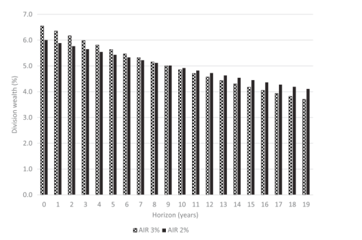
We investigate variable annuities, where the variability arises due to risky investment returns. We study the relationship between the so-called assumed interest rate (AIR) and the (expected) annuity payments. The AIR effectively determines the decumulation speed of financial wealth over the payout phase: a larger AIR leads to higher early payments and lower later payments. In case the AIR equals the expected return on the underlying portfolio, the income during the payout phase is, in expectation, constant. See Dellinger (2006) and Horneff et al. (2010) for more details on the usage of the AIR concept in insurance pricing. We provide a novel way to solve the optimal consumption problem and, in doing so, derive the AIR that optimizes lifetime utility of consumption. We also analyze the utility loss of investors with constant relative risk aversion (CRRA) preferences who allocate their wealth suboptimally over their life cycle and/or have a suboptimal risk exposure. Under the assumption of an optimally chosen risk exposure, we find that a restriction to a (suboptimal) constant expected pension income does not lead to large utility losses. We also show that pension payments with a horizon of “only” 10 years are fairly insensitive to the choice of the AIR. As a result, unlike common practice, communication about the effect of choosing an AIR is preferably based on results for horizons closer to 20 years. We also investigate how financial shocks can be smoothed and what the effect is on the variable annuity. In that case, we find that a horizon-dependent AIR ensures a constant expected pension income.
数学代考|金融数学代考Financial Mathematics代写|VARIABLE ANNUITIES
The financial market that we consider is described by the seminal work of Merton (1971). This implies that in the standard Black-Scholes/Merton setting there is a risk-free asset with a constant interest rate $r$, there is a risky asset with price $\mathrm{St}$ at time t that evolves by the diffusion process.
$$
\begin{aligned}
\mathrm{d} S_{t} &=\mu S_{t} \mathrm{~d} t+\sigma S_{t} \mathrm{~d} Z_{t} \
&=(r+\lambda \sigma) S_{l} \mathrm{~d} t+\sigma S_{l} \mathrm{~d} Z_{t} .
\end{aligned}
$$
Thus, we assume that the stock price $S_{t}$ follows a geometric Brownian motion, where $\mu$ stands for the expected return, $\sigma$ is the stock volatility, $\lambda$ is the Sharpe ratio
$$
\lambda=(\mu-r) / \sigma,
$$
and $Z$ is a standard Brownian motion on the probability space $(\Omega, F, P)$
Moreover, we assume the isoelastic (power) function for utility that exhibits a CRRA and is given by
$$
u(x)= \begin{cases}\frac{x^{1-\gamma}}{1-\gamma} & \text { if } \gamma>0, \gamma \neq 1 \ \ln (x) & \text { if } \gamma=1\end{cases}
$$
where $\gamma$ is the relative risk aversion level. The more risk averse the investor is, the higher $\gamma$. We exclude negative risk aversion levels which would imply risk loving preferences. Since additive constant terms in objective functions do not affect optimal decisions, a term of minus one is omitted from the numerator which would be needed to show that the limiting case of $\gamma$ to one converges to logarithmic utility,
In general, the investor is endowed with initial wealth $\mathrm{W}{0}$ which can be used for consumption and the remainder is invested in the financial market. The wealth process is given by $$ \mathrm{d} W{t}=\left(\left(r+w_{t}(\mu-r)\right) W_{t}-c_{t}\right) \mathrm{d} t+\sigma w_{t} W_{t} \mathrm{~d} Z_{t},
$$
where $w_{t}$ is the fraction invested in the risky asset and $c_{t}$ is the withdrawal
(consumption) rate. For the CRRA utility function, the optimal time-varying risk exposure $w_{t}$ is known to be
$$
w^{*}=\frac{\lambda}{\gamma \sigma} ;
$$
see, for example Theorem 3.8.8. in Karatzas and Shreve (1998). That is, the optimal exposure is state- and time-independent. Concerning the optimal consumption choice, we represent the withdrawal via the AIR which determines the allocation of initial wealth to the (optimal) consumption at various horizons. We formulate this problem using a discrete number of consumption dates which effectively means that we solve H separate terminal wealth problems. The novelty in this setup allows us to directly cast optimal consumption questions into AIRs in variable annuities.
As an example, consider a retiree who enters retirement with total wealth $\mathrm{W}_{0}$ at time 0 and who needs to finance $\mathrm{H}$ annual pension payments at times. For ease of exposition, we assume $\mathrm{H}$ to be given; that is, we consider fixed term instead of lifelong variable annuities. Think of $\mathrm{H}$ as the remaining life expectancy at retirement age. ${ }^{2}$
The pension payments at each horizon $\mathrm{h}=0, \ldots, \mathrm{H}-1$ have to be financed from the initial total pension wealth $\mathrm{W}_{0}$. This simple idea is formalized by the notation in the next definition.
金融数学代考
数学代考|金融数学代考Financial Mathematics代写|Human Development in Brazil
本小节介绍了 Cohen (2011) 的结果以及本研究结果的实际应用。这是使用巴西人类发展地图集 (Programa das Nações Unidas para o Desenvolvimento Humano, 2013a) 中的信息计算 e40 和 e60 的界限。出生时的预期寿命是主要的长寿指标,通常用作指标人类发展(Mayhew & Smith, 2015)。由于它们的重要性,出生时预期寿命的数据通常在人口学、公共卫生等研究中列出。但是,当没有关于死亡率的详细数据时,对于其他年龄的预期寿命来说,这种可用性并不容易。Mathers、Stevens、Boerma、White 和 Tobias(2015 年)指出,例如,60 岁时的预期寿命,X,只知道一个人变老的概率X活到老X+n和年龄的完整预期寿命X+n. 当然,使用相同的参数,界限为和X+n是通过先验知识构建的npX和前。也就是说,直接从(8)得出:
e˙\AAX−nnpX≤和˙X+n≤和˙XnpX−n.
巴西人类发展地图集(Programa das Nações Unidas para o Desenvolvimento Humano,2013b)是获取 1991、2000 和 2010 年市政人类发展指数的工具,可在 Programa das Nações Unidas para o Desenvolvimento Humano (2013a)。例如,使用此工具,可以获得有关出生时预期寿命、新生儿存活到 40 岁的概率以及新生儿存活到 60 岁的概率等信息年,适用于所有巴西城市。值得注意的是,2010年,巴西有5565个自治市。因此,可以为巴西各城市在相应年份构建 40 岁和 60 岁的预期寿命值区间,例如,表 5 显示了和40和和602010 年巴西出生时预期寿命最长的 10 个城市。奇怪的是,所有这些城市都属于圣卡塔琳娜州。数据收集于 2017 年 12 月 22 日的巴西人类发展地图集 Programa das Nações Unidas para o Desenvolvimento Humano, 2013a)。
数学代考|金融数学代考Financial Mathematics代写|INTRODUCTION
在过去的几十年中,固定收益养老金计划已在很大程度上转变为没有或较低保障的固定缴款养老金计划。尤其是最近的金融危机和不断增长的预期寿命影响了包括担保在内的养老金制度的可持续性。因此,市场上越来越多的产品明确让这些风险由个人承担,而不是由个人承担。
雇主或保险人。如果递减阶段的养老金支付包含风险,我们将这些设计称为可变年金。固定年金是指支付不确定的年金。
有大量关于可变年金的文献,包括调查不同的嵌入式担保(Mahayni 和 Schneider,2012;Chen 等人,2015 年)、定价可变年金(Bauer 等人,2008 年;Bacinello 等人,2011 年;Nirmalendran 等人。 , 2014)、对冲可变年金 (Coleman et al., 2006; Trottier et al., 2018) 或这些的组合 (Kling et al., 2011; Bernard et al., 2014)。此外,还研究了对不同年金产品的最佳需求(Horneff et al., 2009; Blake et al., 2014; Peijnenburg et al., 2016)。例如,Koijen 等人的研究表明,将股权风险纳入年金产品的设计可以增加福利。(2011)。
我们研究可变年金,其中可变性是由于风险投资回报而产生的。我们研究了所谓的假设利率(AIR)和(预期的)年金支付之间的关系。AIR 有效地决定了支付阶段金融财富的累积速度:更大的 AIR 导致更高的早期支付和更低的后期支付。如果 AIR 等于基础投资组合的预期回报,则支付阶段的收入预期是恒定的。参见 Dellinger (2006) 和 Horneff 等人。(2010) 了解更多关于在保险定价中使用 AIR 概念的详细信息。我们提供了一种解决最优消耗问题的新方法,并由此推导出优化生命周期消耗效用的 AIR。我们还分析了具有恒定相对风险厌恶 (CRRA) 偏好的投资者的效用损失,这些投资者在其生命周期中分配财富不理想和/或风险敞口不理想。在最优选择风险敞口的假设下,我们发现对(次优)恒定预期养老金收入的限制不会导致巨大的效用损失。我们还表明,“仅”10 年的养老金支付对 AIR 的选择相当不敏感。因此,与通常的做法不同,关于选择 AIR 效果的沟通最好基于接近 20 年的结果。我们还研究了如何平滑金融冲击以及对可变年金的影响。在这种情况下,我们发现依赖于地平线的 AIR 确保了预期的养老金收入不变。
数学代考|金融数学代考Financial Mathematics代写|VARIABLE ANNUITIES
Merton (1971) 的开创性著作描述了我们所考虑的金融市场。这意味着在标准 Black-Scholes/Merton 设置中,存在利率不变的无风险资产r, 存在有价格的风险资产小号吨在时间 t 由扩散过程演变。
d小号吨=μ小号吨 d吨+σ小号吨 d从吨 =(r+λσ)小号l d吨+σ小号l d从吨.
因此,我们假设股票价格小号吨遵循几何布朗运动,其中μ代表预期回报,σ是股票波动率,λ是夏普比率
λ=(μ−r)/σ,
和从是概率空间上的标准布朗运动(Ω,F,磷)
此外,我们假设效用的等弹性(幂)函数表现出 CRRA,并由下式给出
在(X)={X1−C1−C 如果 C>0,C≠1 ln(X) 如果 C=1
在哪里C是相对风险厌恶水平。投资者风险厌恶程度越高,C. 我们排除了暗示风险偏好的负面风险厌恶水平。由于目标函数中的加性常数项不影响最优决策,因此分子中省略了一项减一,这将需要表明C到一个收敛到对数效用,
一般来说,投资者被赋予初始财富在0可用于消费,剩余部分投资于金融市场。财富过程由下式给出
d在吨=((r+在吨(μ−r))在吨−C吨)d吨+σ在吨在吨 d从吨,
在哪里在吨是投资于风险资产的部分,并且C吨是撤回
(消费)率。对于 CRRA 效用函数,最佳时变风险敞口在吨已知是
在∗=λCσ;
例如,参见定理 3.8.8。在 Karatzas 和 Shreve (1998)。也就是说,最佳曝光与状态和时间无关。关于最优消费选择,我们表示通过 AIR 的提款,它决定了初始财富在不同时期的(最优)消费的分配。我们使用离散数量的消费日期来制定这个问题,这实际上意味着我们解决了 H 个独立的终端财富问题。这种设置的新颖性使我们能够直接将最佳消费问题转换为可变年金的 AIR。
举个例子,考虑一个退休的退休人员,他拥有全部财富在0在时间 0 和谁需要融资H有时每年支付养老金。为了便于说明,我们假设H给予; 也就是说,我们考虑固定期限而不是终身可变年金。考虑到H作为退休年龄的剩余预期寿命。2
每个层次的养老金支付H=0,…,H−1必须从最初的总养老金财富中筹集资金在0. 这个简单的想法由下一个定义中的符号形式化。

统计代写请认准statistics-lab™. statistics-lab™为您的留学生涯保驾护航。
金融工程代写
金融工程是使用数学技术来解决金融问题。金融工程使用计算机科学、统计学、经济学和应用数学领域的工具和知识来解决当前的金融问题,以及设计新的和创新的金融产品。
非参数统计代写
非参数统计指的是一种统计方法,其中不假设数据来自于由少数参数决定的规定模型;这种模型的例子包括正态分布模型和线性回归模型。
广义线性模型代考
广义线性模型(GLM)归属统计学领域,是一种应用灵活的线性回归模型。该模型允许因变量的偏差分布有除了正态分布之外的其它分布。
术语 广义线性模型(GLM)通常是指给定连续和/或分类预测因素的连续响应变量的常规线性回归模型。它包括多元线性回归,以及方差分析和方差分析(仅含固定效应)。
有限元方法代写
有限元方法(FEM)是一种流行的方法,用于数值解决工程和数学建模中出现的微分方程。典型的问题领域包括结构分析、传热、流体流动、质量运输和电磁势等传统领域。
有限元是一种通用的数值方法,用于解决两个或三个空间变量的偏微分方程(即一些边界值问题)。为了解决一个问题,有限元将一个大系统细分为更小、更简单的部分,称为有限元。这是通过在空间维度上的特定空间离散化来实现的,它是通过构建对象的网格来实现的:用于求解的数值域,它有有限数量的点。边界值问题的有限元方法表述最终导致一个代数方程组。该方法在域上对未知函数进行逼近。[1] 然后将模拟这些有限元的简单方程组合成一个更大的方程系统,以模拟整个问题。然后,有限元通过变化微积分使相关的误差函数最小化来逼近一个解决方案。
tatistics-lab作为专业的留学生服务机构,多年来已为美国、英国、加拿大、澳洲等留学热门地的学生提供专业的学术服务,包括但不限于Essay代写,Assignment代写,Dissertation代写,Report代写,小组作业代写,Proposal代写,Paper代写,Presentation代写,计算机作业代写,论文修改和润色,网课代做,exam代考等等。写作范围涵盖高中,本科,研究生等海外留学全阶段,辐射金融,经济学,会计学,审计学,管理学等全球99%专业科目。写作团队既有专业英语母语作者,也有海外名校硕博留学生,每位写作老师都拥有过硬的语言能力,专业的学科背景和学术写作经验。我们承诺100%原创,100%专业,100%准时,100%满意。
随机分析代写
随机微积分是数学的一个分支,对随机过程进行操作。它允许为随机过程的积分定义一个关于随机过程的一致的积分理论。这个领域是由日本数学家伊藤清在第二次世界大战期间创建并开始的。
时间序列分析代写
随机过程,是依赖于参数的一组随机变量的全体,参数通常是时间。 随机变量是随机现象的数量表现,其时间序列是一组按照时间发生先后顺序进行排列的数据点序列。通常一组时间序列的时间间隔为一恒定值(如1秒,5分钟,12小时,7天,1年),因此时间序列可以作为离散时间数据进行分析处理。研究时间序列数据的意义在于现实中,往往需要研究某个事物其随时间发展变化的规律。这就需要通过研究该事物过去发展的历史记录,以得到其自身发展的规律。
回归分析代写
多元回归分析渐进(Multiple Regression Analysis Asymptotics)属于计量经济学领域,主要是一种数学上的统计分析方法,可以分析复杂情况下各影响因素的数学关系,在自然科学、社会和经济学等多个领域内应用广泛。
MATLAB代写
MATLAB 是一种用于技术计算的高性能语言。它将计算、可视化和编程集成在一个易于使用的环境中,其中问题和解决方案以熟悉的数学符号表示。典型用途包括:数学和计算算法开发建模、仿真和原型制作数据分析、探索和可视化科学和工程图形应用程序开发,包括图形用户界面构建MATLAB 是一个交互式系统,其基本数据元素是一个不需要维度的数组。这使您可以解决许多技术计算问题,尤其是那些具有矩阵和向量公式的问题,而只需用 C 或 Fortran 等标量非交互式语言编写程序所需的时间的一小部分。MATLAB 名称代表矩阵实验室。MATLAB 最初的编写目的是提供对由 LINPACK 和 EISPACK 项目开发的矩阵软件的轻松访问,这两个项目共同代表了矩阵计算软件的最新技术。MATLAB 经过多年的发展,得到了许多用户的投入。在大学环境中,它是数学、工程和科学入门和高级课程的标准教学工具。在工业领域,MATLAB 是高效研究、开发和分析的首选工具。MATLAB 具有一系列称为工具箱的特定于应用程序的解决方案。对于大多数 MATLAB 用户来说非常重要,工具箱允许您学习和应用专业技术。工具箱是 MATLAB 函数(M 文件)的综合集合,可扩展 MATLAB 环境以解决特定类别的问题。可用工具箱的领域包括信号处理、控制系统、神经网络、模糊逻辑、小波、仿真等。