如果你也在 怎样代写决策树decision tree这个学科遇到相关的难题,请随时右上角联系我们的24/7代写客服。
决策树是一种决策支持工具,它使用决策及其可能后果的树状模型,包括偶然事件结果、资源成本和效用。它是显示一个只包含条件控制语句的算法的一种方式。
statistics-lab™ 为您的留学生涯保驾护航 在代写决策树decision tree方面已经树立了自己的口碑, 保证靠谱, 高质且原创的统计Statistics代写服务。我们的专家在代写决策树decision tree代写方面经验极为丰富,各种代写决策树decision tree相关的作业也就用不着说。
我们提供的决策树decision tree及其相关学科的代写,服务范围广, 其中包括但不限于:
- Statistical Inference 统计推断
- Statistical Computing 统计计算
- Advanced Probability Theory 高等概率论
- Advanced Mathematical Statistics 高等数理统计学
- (Generalized) Linear Models 广义线性模型
- Statistical Machine Learning 统计机器学习
- Longitudinal Data Analysis 纵向数据分析
- Foundations of Data Science 数据科学基础
机器学习代写|决策树作业代写decision tree代考|Other Classification Criteria
In this category, we include all criteria that did not fit in the previously-mentioned categories.
Li and Dubes [62] propose a binary criterion for binary-class problems called permutation statistic. It evaluates the degree of similarity between two vectors, $V_{a_{i}}$ and $y$, and the larger this statistic, the more alike the vectors. Vector $V_{a_{i}}$ is calculated as follows. Let $a_{i}$ be a given numeric attribute with the values $[8.20,7.3,9.35,4.8,7.65,4.33]$ and $N_{x}=6$. Vector $y=[0,0,1,1,0,1]$ holds the corresponding class labels. Now consider a given threshold $\Delta=5.0$. Vector $V_{a_{i}}$ is calculated in two steps: first, attribute $a_{i}$ values are sorted, i.e., $a_{i}=$ $[4.33,4.8,7.3,7.65,8.20,9.35]$, consequently rearranging $y=[1,1,0,0,0,1] ;$ then, $V_{a_{i}}(n)$ takes 0 when $a_{i}(n) \leq \Delta$, and 1 otherwise. Thus, $V_{a_{i}}=[0,0,1,1,1,1]$. The permutation statistic first analyses how many $1-1$ matches $(d)$ vectors $V_{a_{i}}$ and $y$ have. In this particular example, $d=1$. Next, it counts how many l’s there are in $V_{a_{i}}\left(n_{a}\right)$ and in $y\left(n_{y}\right)$. Finally, the permutation statistic can be computed as:
$$
\begin{aligned}
\beta^{\text {permutation }}\left(V_{a_{i}}, y\right) &=\sum_{j=0}^{d} \frac{\left(\begin{array}{c}
n_{a} \
j
\end{array}\right)\left(\begin{array}{c}
N_{x}-n_{a} \
n_{y}-j
\end{array}\right)}{\left(\begin{array}{c}
N_{x} \
n_{y}
\end{array}\right)}-\frac{\left(\begin{array}{c}
n_{a} \
d
\end{array}\right)\left(\begin{array}{c}
N_{x}-n_{a} \
n_{y}-d
\end{array}\right)}{\left(\begin{array}{c}
N_{x} \
n_{g}
\end{array}\right)} U \
\left(\begin{array}{c}
n \
m
\end{array}\right) &=0 \text { if } n<0 \text { or } m<0 \text { or } n<m \
&=\frac{n !}{m !(n-m) !} \text { otherwise }
\end{aligned}
$$
where $U$ is a (continuous) random variable distributed uniformly over $[0,1]$.
机器学习代写|决策树作业代写decision tree代考|Regression Criteria
All criteria presented so far are dedicated to classification problems. For regression problems, where the target variable $y$ is continuous, a common approach is to calculate the mean squared error (MSE) as a splitting criterion:
$$
\operatorname{MSE}\left(a_{i}, \mathbf{X}, y\right)=N_{x}^{-1} \sum_{j=1}^{\left|a_{i}\right|} \sum_{x_{l} \in v_{j}}\left(y\left(x_{l}\right)-\overline{v_{v}}\right)^{2}
$$
where $\overline{y_{v}}=N_{v_{i},}^{-1} \sum_{x_{i} \in v_{j}} y\left(x_{l}\right)$. Just as with clustering, we are trying to minimize the within-partition variance. Usually, the sum of squared errors is weighted over each partition according to the estimated probability of an instance belonging to the given partition [12]. Thus, we should rewrite MSE to:
$$
w \operatorname{MSE}\left(a_{i}, \mathbf{X}, y\right)=\sum_{j=1}^{\left|a_{l}\right|} p_{v_{j}}, \sum_{x_{l} \in v_{j}}\left(y\left(x_{l}\right)-\overline{y_{v_{j}}}\right)^{2}
$$
Another common criterion for regression is the sum of absolute deviations (SAD) [12], or similarly its weighted version given by:
$$
w S A D\left(a_{i}, \mathbf{X}, y\right)=\sum_{j=1}^{\left|a_{i}\right|} p_{v j \cdot \bullet} \sum_{x_{l} \in v_{j}} a b s\left(y\left(x_{l}\right)-\operatorname{median}\left(y_{v j}\right)\right)
$$
where median $\left(y_{v_{j}}\right)$ is the target attribute’s median of instances belonging to $\mathbf{X}{\mathrm{a}{i}=\mathbf{v}{\text {}}}$. Quinlan [93] proposes the use of the standard deviation reduction (SDR) for his pioneering system of model trees induction, M5. Wang and Witten [124] extend the work of Quinlan in their proposed system M5′, also employing the SDR criterion. It is given by: $$ \operatorname{SDR}\left(a{i}, \mathbf{X}, y\right)=\sigma_{X}-\sum_{j=1}^{\left|a_{i}\right|} p_{v_{j}, \bullet} \sigma_{v j}
$$
where $\sigma_{X}$ is the standard deviation of instances in $\mathbf{X}$ and $\sigma_{v_{j}}$ the standard deviation of instances in $\mathbf{X}{\mathbf{a}{l}=\mathbf{v}{j}}$. SDR should be maximized, i.e., the weighted sum of standard deviations of each partition should be as small as possible. Thus, partitioning the instance space according to a particular attribute $a{i}$ should provide partitions whose target attribute variance is small (once again we are interested in minimizing the within-partition variance). Observe that minimizing the second term in SDR is equivalent to minimizing wMSE, but in SDR we are using the partition standard deviation $(\sigma)$ as a similarity criterion whereas in wMSE we are using the partition variance $\left(\sigma^{2}\right)$.
机器学习代写|决策树作业代写decision tree代考|Multivariate Splits
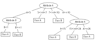
All criteria presented so far are intended for building univariate splits. Decision trees with multivariate splits (known as oblique, linear or multivariate decision trees) are not so popular as the univariate ones, mainly because they are harder to interpret. Nevertheless, researchers reckon that multivariate splits can improve the performance
of the tree in several data sets, while generating smaller trees $[47,77,98]$. Clearly, there is a tradeoff to consider in allowing multivariate tests: simple tests may result in large trees that are hard to understand, yet multivariate tests may result in small trees with tests hard to understand [121].
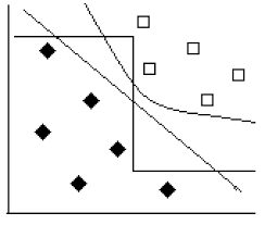
A decision tree with multivariate splits is able to produce polygonal (polyhedral) partitions of the attribute space (hyperplanes at an oblique orientation to the attribute axes) whereas univariate trees can only produce hyper-rectangles parallel to the attribute axes. The tests at each node have the form:
$$
w_{0}+\sum_{i=1}^{n} w_{i} a_{i}(x) \leq 0
$$
where $w_{i}$ is a real-valued coefficient associated to the $i$ th attribute and $w_{0}$ the disturbance coefficient of the test.
CART (Classification and Regression Trees) [12] is one of the first systems that allowed multivariate splits. It employs a hill-climbing strategy with a backward attribute elimination for finding good (albeit suboptimal) linear combinations of attributes in non-terminal nodes. It is a fully-deterministic algorithm with no built-in mechanisms to escape local-optima. Breiman et al. [12] point out that the proposed algorithm has much room for improvement.
Another approach for building oblique decision trees is LMDT (Linear Machine Decision Trees) $[14,119]$, which is an evolution of the perceptron tree method [117]. Each non-terminal node holds a linear machine [83], which is a set of $k$ linear discriminant functions that are used collectively to assign an instance to one of the $k$ existing classes. LMDT uses heuristics to determine when a linear machine has stabilized (since convergence cannot be guaranteed). More specifically, for handling non-linearly separable problems, a method similar to simulated annealing (SA) is used (called thermal training). Draper and Brodley [30] show how LMDT can be altered to induce decision trees that minimize arbitrary misclassification cost functions.
SADT (Simulated Annealing of Decision Trees) [47] is a system that employs SA for finding good coefficient values for attributes in non-terminal nodes of decision trees. First, it places a hyperplane in a canonical location, and then iteratively perturbs the coefficients in small random amounts. At the beginning, when the temperature parameter of the SA is high, practically any perturbation of the coefficients is accepted regardless of the goodness-of-split value (the value of the utilised splitting criterion). As the SA cools down, only perturbations that improve the goodness-of-split are likely to be allowed. Although SADT can eventually escape from local-optima, its efficiency is compromised since it may consider tens of thousands of hyperplanes in a single node during annealing.
决策树代写
机器学习代写|决策树作业代写decision tree代考|Other Classification Criteria
在此类别中,我们包括了所有不符合上述类别的标准。
Li 和 Dubes [62] 提出了一种二元类问题的二元标准,称为排列统计。它评估两个向量之间的相似程度,在一种一世和是,并且这个统计量越大,向量越相似。向量在一种一世计算如下。让一种一世是具有值的给定数字属性[8.20,7.3,9.35,4.8,7.65,4.33]和ñX=6. 向量是=[0,0,1,1,0,1]持有相应的类标签。现在考虑给定的阈值Δ=5.0. 向量在一种一世计算分两步:首先,属性一种一世值是排序的,即一种一世= [4.33,4.8,7.3,7.65,8.20,9.35],因此重新排列是=[1,1,0,0,0,1];然后,在一种一世(n)取 0 时一种一世(n)≤Δ, 否则为 1。因此,在一种一世=[0,0,1,1,1,1]. 排列统计量首先分析有多少1−1火柴(d)矢量图在一种一世和是有。在这个特定的例子中,d=1. 接下来,它计算有多少 l 有在一种一世(n一种)并且在是(n是). 最后,排列统计量可以计算为:
b排列 (在一种一世,是)=∑j=0d(n一种 j)(ñX−n一种 n是−j)(ñX n是)−(n一种 d)(ñX−n一种 n是−d)(ñX nG)在 (n 米)=0 如果 n<0 或者 米<0 或者 n<米 =n!米!(n−米)! 除此以外
在哪里在是一个(连续的)随机变量,均匀分布在[0,1].
机器学习代写|决策树作业代写decision tree代考|Regression Criteria
到目前为止提出的所有标准都专用于分类问题。对于回归问题,其中目标变量是是连续的,常用的方法是计算均方误差(MSE)作为分割标准:
MSE(一种一世,X,是)=ñX−1∑j=1|一种一世|∑Xl∈在j(是(Xl)−在在¯)2
在哪里是在¯=ñ在一世,−1∑X一世∈在j是(Xl). 就像聚类一样,我们试图最小化分区内的方差。通常,误差平方和根据属于给定分区的实例的估计概率在每个分区上加权 [12]。因此,我们应该将 MSE 重写为:
在MSE(一种一世,X,是)=∑j=1|一种l|p在j,∑Xl∈在j(是(Xl)−是在j¯)2
回归的另一个常见标准是绝对偏差之和 (SAD) [12],或者类似地,其加权版本由下式给出:
在小号一种D(一种一世,X,是)=∑j=1|一种一世|p在j⋅∙∑Xl∈在j一种bs(是(Xl)−中位数(是在j))
其中中位数(是在j)是目标属性属于的实例的中位数X一种一世=在. Quinlan [93] 建议在他的模型树归纳系统 M5 中使用标准差缩减 (SDR)。Wang 和 Witten [124] 在他们提出的系统 M5′ 中扩展了 Quinlan 的工作,也采用了 SDR 标准。它由以下给出:特别提款权(一种一世,X,是)=σX−∑j=1|一种一世|p在j,∙σ在j
在哪里σX是实例的标准差X和σ在j实例的标准差X一种l=在j. SDR 应最大化,即每个分区的标准差的加权和应尽可能小。因此,根据特定属性划分实例空间一种一世应该提供目标属性方差很小的分区(我们再次对最小化分区内方差感兴趣)。观察到最小化 SDR 中的第二项等同于最小化 wMSE,但在 SDR 中,我们使用的是分区标准差(σ)作为相似性标准,而在 wMSE 中,我们使用分区方差(σ2).
机器学习代写|决策树作业代写decision tree代考|Multivariate Splits
到目前为止提出的所有标准都旨在构建单变量拆分。具有多元分裂的决策树(称为倾斜、线性或多元决策树)不像单变量决策树那么受欢迎,主要是因为它们更难解释。尽管如此,研究人员认为多变量拆分可以提高性能
在几个数据集中的树,同时生成更小的树[47,77,98]. 显然,在允许多变量测试时需要考虑权衡:简单的测试可能会导致难以理解的大树,而多变量测试可能会导致测试难以理解的小树 [121]。
具有多元分裂的决策树能够产生属性空间的多边形(多面体)分区(与属性轴倾斜方向的超平面),而单变量树只能产生平行于属性轴的超矩形。每个节点的测试具有以下形式:
在0+∑一世=1n在一世一种一世(X)≤0
在哪里在一世是与相关的实值系数一世属性和在0测试的干扰系数。
CART(分类和回归树)[12] 是最早允许多变量拆分的系统之一。它采用具有后向属性消除的爬山策略,以在非终端节点中找到良好(尽管次优)的属性线性组合。它是一种完全确定的算法,没有内置机制来逃避局部最优。布雷曼等人。[12]指出,所提出的算法有很大的改进空间。
构建倾斜决策树的另一种方法是 LMDT(线性机器决策树)[14,119],这是感知器树方法的演变[117]。每个非终端节点都有一个线性机器[83],它是一组ķ线性判别函数共同用于将实例分配给其中一个ķ现有的类。LMDT 使用启发式方法来确定线性机器何时稳定(因为无法保证收敛)。更具体地说,为了处理非线性可分问题,使用类似于模拟退火 (SA) 的方法(称为热训练)。Draper 和 Brodley [30] 展示了如何更改 LMDT 以诱导决策树,从而最大限度地减少任意错误分类成本函数。
SADT(决策树的模拟退火)[47] 是一个系统,它使用 SA 来为决策树的非终端节点中的属性找到良好的系数值。首先,它将超平面放置在规范位置,然后以小随机量迭代地扰动系数。开始时,当 SA 的温度参数较高时,几乎可以接受系数的任何扰动,而不管分割的优度值(使用的分割标准的值)。随着 SA 冷却下来,可能只允许提高分裂优度的扰动。尽管 SADT 最终可以摆脱局部最优,但它的效率会受到影响,因为它可能会在退火期间考虑单个节点中的数万个超平面。

统计代写请认准statistics-lab™. statistics-lab™为您的留学生涯保驾护航。
金融工程代写
金融工程是使用数学技术来解决金融问题。金融工程使用计算机科学、统计学、经济学和应用数学领域的工具和知识来解决当前的金融问题,以及设计新的和创新的金融产品。
非参数统计代写
非参数统计指的是一种统计方法,其中不假设数据来自于由少数参数决定的规定模型;这种模型的例子包括正态分布模型和线性回归模型。
广义线性模型代考
广义线性模型(GLM)归属统计学领域,是一种应用灵活的线性回归模型。该模型允许因变量的偏差分布有除了正态分布之外的其它分布。
术语 广义线性模型(GLM)通常是指给定连续和/或分类预测因素的连续响应变量的常规线性回归模型。它包括多元线性回归,以及方差分析和方差分析(仅含固定效应)。
有限元方法代写
有限元方法(FEM)是一种流行的方法,用于数值解决工程和数学建模中出现的微分方程。典型的问题领域包括结构分析、传热、流体流动、质量运输和电磁势等传统领域。
有限元是一种通用的数值方法,用于解决两个或三个空间变量的偏微分方程(即一些边界值问题)。为了解决一个问题,有限元将一个大系统细分为更小、更简单的部分,称为有限元。这是通过在空间维度上的特定空间离散化来实现的,它是通过构建对象的网格来实现的:用于求解的数值域,它有有限数量的点。边界值问题的有限元方法表述最终导致一个代数方程组。该方法在域上对未知函数进行逼近。[1] 然后将模拟这些有限元的简单方程组合成一个更大的方程系统,以模拟整个问题。然后,有限元通过变化微积分使相关的误差函数最小化来逼近一个解决方案。
tatistics-lab作为专业的留学生服务机构,多年来已为美国、英国、加拿大、澳洲等留学热门地的学生提供专业的学术服务,包括但不限于Essay代写,Assignment代写,Dissertation代写,Report代写,小组作业代写,Proposal代写,Paper代写,Presentation代写,计算机作业代写,论文修改和润色,网课代做,exam代考等等。写作范围涵盖高中,本科,研究生等海外留学全阶段,辐射金融,经济学,会计学,审计学,管理学等全球99%专业科目。写作团队既有专业英语母语作者,也有海外名校硕博留学生,每位写作老师都拥有过硬的语言能力,专业的学科背景和学术写作经验。我们承诺100%原创,100%专业,100%准时,100%满意。
随机分析代写
随机微积分是数学的一个分支,对随机过程进行操作。它允许为随机过程的积分定义一个关于随机过程的一致的积分理论。这个领域是由日本数学家伊藤清在第二次世界大战期间创建并开始的。
时间序列分析代写
随机过程,是依赖于参数的一组随机变量的全体,参数通常是时间。 随机变量是随机现象的数量表现,其时间序列是一组按照时间发生先后顺序进行排列的数据点序列。通常一组时间序列的时间间隔为一恒定值(如1秒,5分钟,12小时,7天,1年),因此时间序列可以作为离散时间数据进行分析处理。研究时间序列数据的意义在于现实中,往往需要研究某个事物其随时间发展变化的规律。这就需要通过研究该事物过去发展的历史记录,以得到其自身发展的规律。
回归分析代写
多元回归分析渐进(Multiple Regression Analysis Asymptotics)属于计量经济学领域,主要是一种数学上的统计分析方法,可以分析复杂情况下各影响因素的数学关系,在自然科学、社会和经济学等多个领域内应用广泛。
MATLAB代写
MATLAB 是一种用于技术计算的高性能语言。它将计算、可视化和编程集成在一个易于使用的环境中,其中问题和解决方案以熟悉的数学符号表示。典型用途包括:数学和计算算法开发建模、仿真和原型制作数据分析、探索和可视化科学和工程图形应用程序开发,包括图形用户界面构建MATLAB 是一个交互式系统,其基本数据元素是一个不需要维度的数组。这使您可以解决许多技术计算问题,尤其是那些具有矩阵和向量公式的问题,而只需用 C 或 Fortran 等标量非交互式语言编写程序所需的时间的一小部分。MATLAB 名称代表矩阵实验室。MATLAB 最初的编写目的是提供对由 LINPACK 和 EISPACK 项目开发的矩阵软件的轻松访问,这两个项目共同代表了矩阵计算软件的最新技术。MATLAB 经过多年的发展,得到了许多用户的投入。在大学环境中,它是数学、工程和科学入门和高级课程的标准教学工具。在工业领域,MATLAB 是高效研究、开发和分析的首选工具。MATLAB 具有一系列称为工具箱的特定于应用程序的解决方案。对于大多数 MATLAB 用户来说非常重要,工具箱允许您学习和应用专业技术。工具箱是 MATLAB 函数(M 文件)的综合集合,可扩展 MATLAB 环境以解决特定类别的问题。可用工具箱的领域包括信号处理、控制系统、神经网络、模糊逻辑、小波、仿真等。