如果你也在 怎样代写光学Optics这个学科遇到相关的难题,请随时右上角联系我们的24/7代写客服。
光学是研究光的行为和属性的物理学分支,包括它与物质的相互作用以及使用或探测它的仪器的构造。光学通常描述可见光、紫外光和红外光的行为。
statistics-lab™ 为您的留学生涯保驾护航 在代写光学Optics方面已经树立了自己的口碑, 保证靠谱, 高质且原创的统计Statistics代写服务。我们的专家在代写光学Optics代写方面经验极为丰富,各种代写光学Optics相关的作业也就用不着说。
我们提供的光学Optics及其相关学科的代写,服务范围广, 其中包括但不限于:
- Statistical Inference 统计推断
- Statistical Computing 统计计算
- Advanced Probability Theory 高等概率论
- Advanced Mathematical Statistics 高等数理统计学
- (Generalized) Linear Models 广义线性模型
- Statistical Machine Learning 统计机器学习
- Longitudinal Data Analysis 纵向数据分析
- Foundations of Data Science 数据科学基础
物理代写|光学代写Optics代考|Cloak for Perfect Conductor
The cloaks for perfect conductor are inversely designed using the developed method. This is a typical min-type optimization problem. Topology optimization-based inverse design of two-dimensional optical cloaks have been investigated for transverse magnetic and transverse electric incident waves, where two-dimensional is the reduced case with an infinite extension assumed in the third dimension $[3,4$, 16]. Three-dimensional design is more flexible and practical for the consideration of realistic situations.
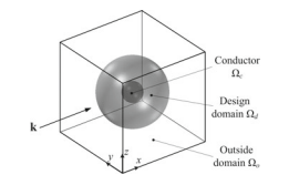
In the following, optical cloaks are designed for a spherical perfect conductor. To cloak the sphere, the scattering field should be minimized to achieve phase matching of the total field around the conductor. The inverse domain of the cloak is set to be a cube with side length equal to 7 times the incident wavelength, as shown in Fig. 3.3, where the cloak domain is set to be a spherical shell with external and internal radii equal to $2.5$ and $0.75$ times the incident wavelength, and the cloaked conductor is enclosed in a central spherical domain with a radius equal to $0.75$ times the incident wavelength. The computational domain is discretized by $63 \times 63 \times 63$ brick elements.
For a magnetic field described optical cloak, the objective in Eq.3.8 is set to minimize the normalized square norm of the scattered magnetic field
$$
J=\frac{1}{J_{0}} \int_{\Omega_{a}} \mathbf{H}{s} \cdot \overline{\mathbf{H}}{s} \mathrm{~d} \Omega
$$
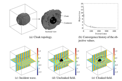
where $\Omega_{o}$ is the domain outside the spherical shell-shaped design domain; $J_{0}$ is the square norm of the uncloaked scattered magnetic field in the outside domain of the cloak. The obtained cloak topology, found by solving the corresponding topology optimization problem, is shown in Fig. 3.4a, with incident wave, uncloaked field, and cloaked field shown in Fig. $3.4 \mathrm{c}, \mathrm{d}$, and $\mathrm{e}$, where the incident wave is set to be the
uniform plane wave $\mathbf{H}{i}=\left(0,0, e^{-j k{0} x}\right)$ with $k_{0}=20 \pi \mathrm{rad} / \mathrm{m}$. For an electric field described optical cloak, the objective in Eq. $3.24$ is set to minimize the normalized square norm of the scattered electric field
$$
J=\frac{1}{J_{0}} \int_{\Omega_{o}} \mathbf{E}{s} \cdot \overline{\mathbf{E}}{s} \mathrm{~d} \Omega
$$
where $J_{0}$ is the square norm of the uncloaked scattered electric field in the outside domain of the cloak. The obtained cloak topology, found by solving the corresponding topology optimization problem, is shown in Fig. 3.5a, with incident wave, uncloaked field, and cloaked field respectively shown in Fig. $3.5 \mathrm{c}, \mathrm{d}$, and e, where the incident wave is set to be the uniform plane wave $\mathbf{E}{i}=\left(0,0, e^{-j k{0} x}\right)$ with $k_{0}=20 \pi \mathrm{rad} / \mathrm{m}$. Objective convergent histories for both these two cases were respectively plotted in Fig. 3.4b and b, which has demonstrated the robustness of the convergent process of the solving procedure.
The inversely designed cloaks have effectively reduced the scattering energy in the outside domain of the cloaks, and this can be confirmed by comparing the uncloaked and cloaked fields shown in Figs. $3.4 \mathrm{~d}$ and e, $3.5 \mathrm{~d}$ and e.
物理代写|光学代写Optics代考|Dielectric Resonator
This section considers max-type optimization problems, for which dielectric-based optical resonator design is a typical task. Optical resonators are designed to concentrate the optical energy in a specified spherical domain, where the total field should be maximized, hence achieving a resonance of the total field in this domain. The computational domain of the resonator is set to be a cube with side length equal to $2.5$ times the incident wavelength, as shown in Fig. 3.7, where the design domain is set to be a spherical shell with external and internal radii respectively equal to 1 and
$0.3$ times the incident wavelength, and the resonating domain is the central spherical domain with radius equal to $0.3$ times the incident wavelength. The computational domain is discretized by $50 \times 50 \times 50$ brick elements.
For the magnetic field described case, the objective in Eq. $3.8$ is set to maximize the normalized square norm of the total magnetic field in the resonating domain
$$
J=\frac{1}{J_{0}} \int_{\Omega_{r}} \mathbf{H} \cdot \overline{\mathbf{H}} \mathrm{d} \Omega
$$
where $\Omega_{r}$ is the resonating domain; $J_{0}$ is the square norm of the total magnetic field in the resonating domain, with dielectric filled in the design domain. After implementing the solution procedure introduced in Sect. 3.1.5, the obtained resonator topology is shown in Fig. 3.8a, with incident wave and resonating field shown in Fig. 3.8c and d, and in which the incident field is set to be the uniform plane wave $\mathbf{H}{i}=\left(0,0, e^{-j k{0} x}\right)$ with $k_{0}=20 \pi \mathrm{rad} / \mathrm{m}$. For the electric field described case, the objective in Eq. $3.24$ is set to maximize the normalized square norm of the total electric field in the resonating domain
$$
J=\frac{1}{J_{0}} \int_{\Omega_{r}} \mathbf{E} \cdot \overline{\mathbf{E}} \mathrm{d} \Omega
$$
where $J_{0}$ is the square norm of the electric field in the resonating domain, with dielectric filled in the design domain. The obtained resonator topology is shown in Fig. 3.9a, with incident wave and resonating field respectively shown in Fig. $3.9 \mathrm{c}$ and $\mathrm{d}$, where the incident wave is set to be the uniform plane wave $\mathbf{E}{i}=\left(0,0, e^{-j k{0} x}\right)$ with $k_{0}=20 \pi \mathrm{rad} / \mathrm{m}$. The objective convergent histories for both cases are plotted in Figs. $3.8 \mathrm{~b}$ and $3.9 \mathrm{~b}$, and demonstrate the robustness of the convergence process of the solution procedure. The computationally designed resonators have effectively focused the optical energy in the resonating domain of the resonator, where the optical field has been enhanced effectively; and this can be confirmed by inspecting the field distribution shown in Figs. $3.8 \mathrm{~d}$ and $3.9 \mathrm{~d}$.
To check the optimality of the derived resonator topologies in Figs. $3.8 \mathrm{a}$ and $3.9 \mathrm{a}$, the similar cross comparison method is adopted as that in Sect. 3.2.1. By exchanging the corresponding incident waves, the magnetic field distribution around the resonator in Fig. 3.9a induced by the incident wave in Fig. 3.8c is shown in Fig. 3.10a; and electric field distribution around the resonator in Fig. 3.8a induced by the incident wave in Fig. 3.9c is shown in Fig. 3.10b. The objective values corresponding to Figs. $3.8 \mathrm{~d}$ and $3.10 \mathrm{a}, 3.9 \mathrm{~d}$ and $3.10 \mathrm{~b}$ are listed in Table 3.2. From the comparison of the values in Table $3.2$, the optimality can be confirmed for the derived resonator topologies in Figs. $3.8 \mathrm{a}$ and $3.9 \mathrm{a}$.
物理代写|光学代写Optics代考|Beam Splitter
An optical splitter is topologically optimized in the following, in order to demonstrate the robustness of the developed method when applied to max-min-type optimization
problems. For computationally designing the splitters, the computational domain is set up as shown in Fig.3.11, where the optical energy enters the domain from the inlet $\Gamma_{i}$ and output from the two specified outlets $\Gamma_{o 1}$ and $\Gamma_{o 2}$. The computational domain is discretized by $60 \times 60 \times 12$ elements. The incident wave is set to be the $z$-polarized uniform plane wave with a frequency equal to $1 \times 10^{9} \mathrm{~Hz}$.
The design objective of the splitter is to achieve equal and maximized energy levels at the two outlets. Therefore, for the magnetic field case, the design objective is set to maximize
$$
\min \left{\int_{\Gamma_{a 1}} \frac{1}{2} \mu_{0} \mu_{r} \mathbf{H} \cdot \overline{\mathbf{H}} \mathrm{d} \Gamma, \int_{\Gamma_{a} 2} \frac{1}{2} \mu_{0} \mu_{r} \mathbf{H} \cdot \overline{\mathbf{H}} \mathrm{d} \Gamma\right}
$$
and for the electric field case, the design objective is modified to maximize
$$
\min \left{\int_{\Gamma_{e 1}} \frac{1}{2} \varepsilon_{0} \varepsilon_{r} \mathbf{E} \cdot \overline{\mathbf{E}} \mathrm{d} \Gamma, \int_{\Gamma_{c 2}} \frac{1}{2} \varepsilon_{0} \varepsilon_{r} \mathbf{E} \cdot \overline{\mathbf{E}} \mathrm{d} \Gamma\right}
$$
The splitter topology is derived as shown in Figs. $3.12$ and $3.13$, where the convergence histories of objective values and field distribution are included. From the field distribution in Figs. $3.12 \mathrm{c}$ and $3.13 \mathrm{c}$, one can confirm by inspection the wave splitting performance of the computationally designed splitters. The splitting and parallelization was achieved in approximately eight wavelengths for both versions.
The optimality of the derived splitter topologies in Figs. 3.12a and $3.13 \mathrm{a}$ is checked with the cross comparison implemented by exchanging the corresponding incident waves. When the splitter in Fig. 3.13a is used for the magnetic wave, the magnetic field is distributed as shown Fig. 3.14a; and when the splitter in Fig. 3.12a is used for the electric field, the electric field is distributed as shown in Fig. 3.14b. The objective values corresponding to Figs. $3.12 \mathrm{c}$ and $3.14 \mathrm{a}, 3.13 \mathrm{c}$ and $3.14 \mathrm{~b}$ are listed in Table $3.3$. From the comparison of the values in Table $3.3$, the optimality for the derived splitter topologies in Figs. 3.12a and 3.13a is confirmed.
光学代考
物理代写|光学代写Optics代考|Cloak for Perfect Conductor
完美导体的斗篷是使用开发的方法逆向设计的。这是一个典型的 min-type 优化问题。已经研究了基于拓扑优化的二维光学斗篷的逆向设计,用于横向磁和横向电入射波,其中二维是在三维假设无限扩展的简化情况[3,4, 16]。立体设计更加灵活实用,考虑到现实情况。
在下文中,光学斗篷是为球形完美导体设计的。为了掩盖球体,散射场应该最小化,以实现导体周围总场的相位匹配。斗篷的逆域设置为边长等于入射波长的 7 倍的立方体,如图 3.3 所示,其中斗篷域设置为外半径和内半径等于的球壳2.5和0.75乘以入射波长,隐形导体被包围在一个半径等于0.75乘以入射波长。计算域离散化为63×63×63砖元素。
对于磁场描述的光学斗篷,Eq.3.8 中的目标设置为最小化散射磁场的归一化平方范数
$$
J=\frac{1}{J_{0}} \int_{\Omega_{a} } \mathbf{H} {s} \cdot \overline{\mathbf{H}} {s} \mathrm{~d} \Omega
$$
其中Ω○是球壳形设计域外的域;Ĵ0是斗篷外域中未隐身散射磁场的平方范数。通过求解相应的拓扑优化问题得到的隐身拓扑如图3.4a所示,入射波、非隐身场和隐身场如图3.4a所示。3.4C,d, 和和,其中入射波设置为
均匀平面波H一世=(0,0,和−jķ0X)和ķ0=20圆周率r一个d/米. 对于电场描述的光学斗篷,方程式中的物镜。3.24设置为最小化散射电场的归一化平方范数
Ĵ=1Ĵ0∫Ω○和s⋅和¯s dΩ
在哪里Ĵ0是隐身外域中未隐身散射电场的平方范数。通过求解相应的拓扑优化问题得到的隐身拓扑如图 3.5a 所示,入射波、非隐身场和隐身场分别如图 3.5a 所示。3.5C,d, 和 e, 其中入射波设置为均匀平面波和一世=(0,0,和−jķ0X)和ķ0=20圆周率r一个d/米. 这两种情况的客观收敛历史分别绘制在图 3.4b 和 b 中,这证明了求解过程收敛过程的鲁棒性。
逆向设计的斗篷有效地降低了斗篷外域的散射能量,这可以通过比较图1和2所示的非隐身场和隐身场来证实。3.4 d和 e,3.5 d和 e。
物理代写|光学代写Optics代考|Dielectric Resonator
本节考虑最大型优化问题,其中基于介质的光学谐振器设计是典型任务。光学谐振器旨在将光能集中在指定的球面域中,其中总场应最大化,从而在该域中实现总场的共振。谐振器的计算域设置为边长等于的立方体2.5乘以入射波长,如图 3.7 所示,其中设计域设置为外半径和内半径分别等于 1 和
0.3乘以入射波长,共振域是中心球域,半径等于0.3乘以入射波长。计算域离散化为50×50×50砖元素。
对于所描述的磁场情况,方程式中的目标。3.8设置为最大化谐振域中总磁场的归一化平方范数
Ĵ=1Ĵ0∫ΩrH⋅H¯dΩ
在哪里Ωr是共振域;Ĵ0是谐振域中总磁场的平方范数,在设计域中填充了电介质。在执行第 3 节中介绍的解决程序后。3.1.5,得到的谐振腔拓扑如图3.8a所示,入射波和谐振场如图3.8c和d所示,其中入射场设置为均匀平面波H一世=(0,0,和−jķ0X)和ķ0=20圆周率r一个d/米. 对于电场描述的情况,方程式中的目标。3.24设置为最大化谐振域中总电场的归一化平方范数
Ĵ=1Ĵ0∫Ωr和⋅和¯dΩ
在哪里Ĵ0是谐振域中电场的平方范数,电介质填充在设计域中。得到的谐振器拓扑如图 3.9a 所示,入射波和谐振场分别如图 3.9a 所示。3.9C和d,其中入射波设置为均匀平面波和一世=(0,0,和−jķ0X)和ķ0=20圆周率r一个d/米. 两种情况的客观收敛历史都绘制在图 1 和图 2 中。3.8 b和3.9 b,并证明求解过程的收敛过程的鲁棒性。计算设计的谐振腔有效地将光能集中在谐振腔的谐振域中,光场得到有效增强;这可以通过检查图 1 和 2 所示的场分布来确认。3.8 d和3.9 d.
为了检查图 1 和 2 中导出的谐振器拓扑的最优性。3.8一个和3.9一个, 采用与 Sect 类似的交叉比较方法。3.2.1。通过交换相应的入射波,图 3.8c 中的入射波在图 3.9a 中谐振器周围感应出的磁场分布如图 3.10a 所示;图 3.9c 中的入射波引起的图 3.8a 中谐振器周围的电场分布如图 3.10b 所示。对应于无花果的客观值。3.8 d和3.10一个,3.9 d和3.10 b列于表 3.2 中。从表中数值的比较3.2,可以确认图 1 和 2 中导出的谐振器拓扑的最优性。3.8一个和3.9一个.
物理代写|光学代写Optics代考|Beam Splitter
下面对分光器进行拓扑优化,以证明所开发方法在应用于 max-min-type 优化时的鲁棒性
问题。为了计算设计分光器,计算域设置如图 3.11 所示,其中光能从入口进入域Γ一世并从两个指定的出口输出Γ○1和Γ○2. 计算域离散化为60×60×12元素。入射波设置为和-偏振均匀平面波,频率等于1×10⁹ H和.
分流器的设计目标是在两个出口处实现相等和最大化的能量水平。因此,对于磁场情况,设计目标设定为最大化
\min \left{\int_{\Gamma_{a 1}} \frac{1}{2} \mu_{0} \mu_{r} \mathbf{H}\cdot\overline{\mathbf{H}}\ mathrm{d}\Gamma,\int_{\Gamma_{a}2}\frac{1}{2}\mu_{0}\mu_{r}\mathbf{H}\cdot\overline{\mathbf{H} } \mathrm{d}\Gamma\right}\min \left{\int_{\Gamma_{a 1}} \frac{1}{2} \mu_{0} \mu_{r} \mathbf{H}\cdot\overline{\mathbf{H}}\ mathrm{d}\Gamma,\int_{\Gamma_{a}2}\frac{1}{2}\mu_{0}\mu_{r}\mathbf{H}\cdot\overline{\mathbf{H} } \mathrm{d}\Gamma\right}
对于电场情况,修改设计目标以最大化
\min \left{\int_{\Gamma_{e 1}} \frac{1}{2} \varepsilon_{0} \varepsilon_{r}\mathbf{E}\cdot\overline{\mathbf{E}}\ mathrm{d} \Gamma, \int_{\Gamma_{c 2}} \frac{1}{2} \productpsilon_{0}\productpsilon_{r}\mathbf{E}\cdot\overline{\mathbf{E} } \mathrm{d}\Gamma\right}\min \left{\int_{\Gamma_{e 1}} \frac{1}{2} \varepsilon_{0} \varepsilon_{r}\mathbf{E}\cdot\overline{\mathbf{E}}\ mathrm{d} \Gamma, \int_{\Gamma_{c 2}} \frac{1}{2} \productpsilon_{0}\productpsilon_{r}\mathbf{E}\cdot\overline{\mathbf{E} } \mathrm{d}\Gamma\right}
分路器拓扑的推导如图 1 和图 2 所示。3.12和3.13,其中包括目标值和场分布的收敛历史。从图中的场分布。3.12C和3.13C,可以通过检查计算设计的分波器的分波性能来确认。两个版本都在大约八个波长中实现了拆分和并行化。
派生的分离器拓扑的最优性在图 3.12a 和3.13一个通过交换相应的入射波实现的交叉比较来检查。当图 3.13a 中的分路器用于磁波时,磁场分布如图 3.14a 所示;当图 3.12a 中的分路器用于电场时,电场分布如图 3.14b 所示。对应于无花果的客观值。3.12C和3.14一个,3.13C和3.14 b列于表中3.3. 从表中数值的比较3.3,图 1 和 2 中派生的分离器拓扑的最优性。3.12a 和 3.13a 得到确认。

统计代写请认准statistics-lab™. statistics-lab™为您的留学生涯保驾护航。
金融工程代写
金融工程是使用数学技术来解决金融问题。金融工程使用计算机科学、统计学、经济学和应用数学领域的工具和知识来解决当前的金融问题,以及设计新的和创新的金融产品。
非参数统计代写
非参数统计指的是一种统计方法,其中不假设数据来自于由少数参数决定的规定模型;这种模型的例子包括正态分布模型和线性回归模型。
广义线性模型代考
广义线性模型(GLM)归属统计学领域,是一种应用灵活的线性回归模型。该模型允许因变量的偏差分布有除了正态分布之外的其它分布。
术语 广义线性模型(GLM)通常是指给定连续和/或分类预测因素的连续响应变量的常规线性回归模型。它包括多元线性回归,以及方差分析和方差分析(仅含固定效应)。
有限元方法代写
有限元方法(FEM)是一种流行的方法,用于数值解决工程和数学建模中出现的微分方程。典型的问题领域包括结构分析、传热、流体流动、质量运输和电磁势等传统领域。
有限元是一种通用的数值方法,用于解决两个或三个空间变量的偏微分方程(即一些边界值问题)。为了解决一个问题,有限元将一个大系统细分为更小、更简单的部分,称为有限元。这是通过在空间维度上的特定空间离散化来实现的,它是通过构建对象的网格来实现的:用于求解的数值域,它有有限数量的点。边界值问题的有限元方法表述最终导致一个代数方程组。该方法在域上对未知函数进行逼近。[1] 然后将模拟这些有限元的简单方程组合成一个更大的方程系统,以模拟整个问题。然后,有限元通过变化微积分使相关的误差函数最小化来逼近一个解决方案。
tatistics-lab作为专业的留学生服务机构,多年来已为美国、英国、加拿大、澳洲等留学热门地的学生提供专业的学术服务,包括但不限于Essay代写,Assignment代写,Dissertation代写,Report代写,小组作业代写,Proposal代写,Paper代写,Presentation代写,计算机作业代写,论文修改和润色,网课代做,exam代考等等。写作范围涵盖高中,本科,研究生等海外留学全阶段,辐射金融,经济学,会计学,审计学,管理学等全球99%专业科目。写作团队既有专业英语母语作者,也有海外名校硕博留学生,每位写作老师都拥有过硬的语言能力,专业的学科背景和学术写作经验。我们承诺100%原创,100%专业,100%准时,100%满意。
随机分析代写
随机微积分是数学的一个分支,对随机过程进行操作。它允许为随机过程的积分定义一个关于随机过程的一致的积分理论。这个领域是由日本数学家伊藤清在第二次世界大战期间创建并开始的。
时间序列分析代写
随机过程,是依赖于参数的一组随机变量的全体,参数通常是时间。 随机变量是随机现象的数量表现,其时间序列是一组按照时间发生先后顺序进行排列的数据点序列。通常一组时间序列的时间间隔为一恒定值(如1秒,5分钟,12小时,7天,1年),因此时间序列可以作为离散时间数据进行分析处理。研究时间序列数据的意义在于现实中,往往需要研究某个事物其随时间发展变化的规律。这就需要通过研究该事物过去发展的历史记录,以得到其自身发展的规律。
回归分析代写
多元回归分析渐进(Multiple Regression Analysis Asymptotics)属于计量经济学领域,主要是一种数学上的统计分析方法,可以分析复杂情况下各影响因素的数学关系,在自然科学、社会和经济学等多个领域内应用广泛。
MATLAB代写
MATLAB 是一种用于技术计算的高性能语言。它将计算、可视化和编程集成在一个易于使用的环境中,其中问题和解决方案以熟悉的数学符号表示。典型用途包括:数学和计算算法开发建模、仿真和原型制作数据分析、探索和可视化科学和工程图形应用程序开发,包括图形用户界面构建MATLAB 是一个交互式系统,其基本数据元素是一个不需要维度的数组。这使您可以解决许多技术计算问题,尤其是那些具有矩阵和向量公式的问题,而只需用 C 或 Fortran 等标量非交互式语言编写程序所需的时间的一小部分。MATLAB 名称代表矩阵实验室。MATLAB 最初的编写目的是提供对由 LINPACK 和 EISPACK 项目开发的矩阵软件的轻松访问,这两个项目共同代表了矩阵计算软件的最新技术。MATLAB 经过多年的发展,得到了许多用户的投入。在大学环境中,它是数学、工程和科学入门和高级课程的标准教学工具。在工业领域,MATLAB 是高效研究、开发和分析的首选工具。MATLAB 具有一系列称为工具箱的特定于应用程序的解决方案。对于大多数 MATLAB 用户来说非常重要,工具箱允许您学习和应用专业技术。工具箱是 MATLAB 函数(M 文件)的综合集合,可扩展 MATLAB 环境以解决特定类别的问题。可用工具箱的领域包括信号处理、控制系统、神经网络、模糊逻辑、小波、仿真等。