如果你也在 怎样代写光学Optics这个学科遇到相关的难题,请随时右上角联系我们的24/7代写客服。
光学是研究光的行为和属性的物理学分支,包括它与物质的相互作用以及使用或探测它的仪器的构造。光学通常描述可见光、紫外光和红外光的行为。
statistics-lab™ 为您的留学生涯保驾护航 在代写光学Optics方面已经树立了自己的口碑, 保证靠谱, 高质且原创的统计Statistics代写服务。我们的专家在代写光学Optics代写方面经验极为丰富,各种代写光学Optics相关的作业也就用不着说。
我们提供的光学Optics及其相关学科的代写,服务范围广, 其中包括但不限于:
- Statistical Inference 统计推断
- Statistical Computing 统计计算
- Advanced Probability Theory 高等概率论
- Advanced Mathematical Statistics 高等数理统计学
- (Generalized) Linear Models 广义线性模型
- Statistical Machine Learning 统计机器学习
- Longitudinal Data Analysis 纵向数据分析
- Foundations of Data Science 数据科学基础
物理代写|光学代写Optics代考|Topology Optimization Problems
Optical wave propagation is described by Maxwell’s equations. In frequency domain, Maxwell’s equations can be transformed into the wave equations. In order to reduce the dispersion error, the scattering field formulation of the wave equations are used with the time-harmonic factor $e^{j \omega t}$, where $j=\sqrt{-1}$ is the imaginary unit, $\omega$ is the angular frequency and $t$ is the time.
For the optical waves that can be reduced into two dimensions, the transverse magnetic waves with polarization perpendicular to the wave plane are the more general cases. This is because that the transverse magnetic waves can both include the description of related physics with dielectrics and noble metal, where the surface plasmonic polaritons can not be included in the transverse electric waves [16]. Therefore, this chapter focuses on the transverse magnetic waves for the two-dimensional cases. Without losing the generality, it can also be extended to the transverse electric waves with the similar procedure. For the transverse magnetic wave, the wave equation is
$$
\nabla \cdot\left[\varepsilon_{r}^{-1} \nabla\left(H_{s z}+H_{i z}\right)\right]+k_{0}^{2} \mu_{r}\left(H_{s z}+H_{i z}\right)=0, \text { in } \Omega
$$
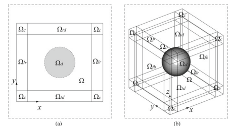
where the transverse magnetic wave is polarized in the $z$-direction; $\nabla$ is the gradient operator in the Cartesian coordinate system; $H_{z}=H_{s z}+H_{i z}$ is the total field, $H_{s z}$ and $H_{i z}$ are the scattering and incident fields, respectively; $\varepsilon_{r}$ and $\mu_{r}$ are the relative permittivity and permeability, respectively; $k_{0}=\omega \sqrt{\varepsilon_{0} \mu_{0}}$ is the free space wave number with $\varepsilon_{0}$ and $\mu_{0}$ respectively representing the permittivity and permeability of the free space; $\Omega$ is a square-shaped wave propagating domain.
For the optical waves that can not be reduced into two dimensions (e.g., optical waves scattered by objects with complicated geometrical configurations), the threedimensional wave equation is used to describe the wave propagation as
$$
\left{\begin{array}{l}
\nabla \times\left[\mu_{r}^{-1} \nabla \times\left(\mathbf{E}{s}+\mathbf{E}{i}\right)\right]-k_{0}^{2} \varepsilon_{r}\left(\mathbf{E}{s}+\mathbf{E}{i}\right)=\mathbf{0}, \text { in } \Omega \
\nabla \cdot\left[\varepsilon_{r}\left(\mathbf{E}{s}+\mathbf{E}{i}\right)\right]=0, \text { in } \Omega
\end{array}\right.
$$
where the electric field $\mathbf{E}=\mathbf{E}{s}+\mathbf{E}{i}$ is the total field, $\mathbf{E}{s}$ and $\mathbf{E}{i}$ are respectively the scattering and incident fields; the second equation is the divergence-free condition of the electric displacement; $\Omega$ is a cuboid-shaped wave propagating domain.
物理代写|光学代写Optics代考|Split of Wave Equations
The iterative procedure is the usual approach to solve the topology optimization problems in Eqs. $2.15$ and 2.16. In the iterative approach, the design variable is evolved based on the gradient information of the cost function. The gradient information can be efficiently derived by the adjoint method [9], which is implemented based on the first-order variational of the augmented Lagrangian of the optimization problems in Eqs. $2.15$ and 2.16. However, the integral functional $A$ of the cost function contains the conjugate of the field variables, which is Gâteaux differential instead of Fréchet differential. This results in the complexity of the adjoint sensitivity, which is self-inconsistent. The self-inconsistency of the sensitivity further results in that the derived structural topology has dependence on the phase of the incident wave. The effect of the self-inconsistent adjoint sensitivity will be demonstrated by the numerical results in Sect. 2.5.1.
To solve the problem on the self-inconsistency of the adjoint sensitivity, the wave equations in Eqs. $2.1$ and $2.2$ can be transformed by splitting the complex variables into the real and imaginary parts. By setting $H_{s z}=H_{s z}^{R}+j H_{s z}^{I}, H_{i z}=H_{i z}^{R}+j H_{i z}^{I}$, $\varepsilon_{r}^{-1}=\left(\varepsilon_{r}^{-1}\right)^{R}+j\left(\varepsilon_{r}^{-1}\right)^{I}$, and substituting these split variables into Eq. 2.1, the twodimensional wave equation is transformed into
$$
\left{\begin{array}{l}
\nabla \cdot\left[\left(\varepsilon_{r}^{-1}\right)^{R} \nabla\left(H_{s z}^{R}+H_{i z}^{R}\right)-\left(\varepsilon_{r}^{-1}\right)^{l} \nabla\left(H_{s z}^{l}+H_{i z}^{l}\right)\right]+k_{0}^{2} \mu_{r}\left(H_{s z}^{R}+H_{i z}^{R}\right)=0, \text { in } \Omega \
\nabla \cdot\left[\left(\varepsilon_{r}^{-1}\right)^{l} \nabla\left(H_{s z}^{R}+H_{i z}^{R}\right)+\left(\varepsilon_{r}^{-1}\right)^{R} \nabla\left(H_{s z}^{l}+H_{i z}^{l}\right)\right]+k_{0}^{2} \mu_{r}\left(H_{s z}^{l}+H_{i z}^{l}\right)=0, \text { in } \Omega
\end{array}\right.
$$
where the superscripts $R$ and $I$ are respectively used to mark the real and imaginary parts of the corresponding complex variable; the scattering boundary conditions for $H_{s z}^{R}$ and $H_{s z}^{I}$ are respectively implemented by solving the split wave equation in the PMLs with complex-valued coordinate transformation and zero-incident field
$$
\left{\begin{array}{l}
\nabla_{\mathbf{x}^{\prime}} \cdot\left[\left(\varepsilon_{r}^{-1}\right)^{R} \nabla_{\mathbf{x}^{\prime}} H_{s z}^{R}-\left(\varepsilon_{r}^{-1}\right)^{l} \nabla_{\mathbf{x}^{\prime}} H_{s z}^{l}\right]+k_{0}^{2} \mu_{r}\left(H_{s z}^{R}+H_{i z}^{R}\right)=0, \text { in } \Omega_{P} \
\nabla_{\mathbf{x}^{\prime}} \cdot\left[\left(\varepsilon_{r}^{-1}\right)^{I} \nabla_{\mathbf{x}^{\prime}} H_{s z}^{R}+\left(\varepsilon_{r}^{-1}\right)^{R} \nabla_{\mathbf{x}^{\prime}} H_{s z}^{l}\right]+k_{0}^{2} \mu_{r}\left(H_{s z}^{l}+H_{i z}^{l}\right)=0, \text { in } \Omega_{P}
\end{array}\right.
$$
Similarly, by setting $\mathbf{E}{s}=\mathbf{E}{s}^{R}+j \mathbf{E}{s}^{l}, \mathbf{E}{i}=\mathbf{E}{i}^{R}+j \mathbf{E}{i}^{l}, \varepsilon_{r}=\varepsilon_{r}^{R}+j \varepsilon_{r}^{l}$, and substituting these split variables into Eq. 2.2, the three-dimensional wave equation is transformed into
$$
\left{\begin{array}{l}
\nabla \times\left[\mu_{r}^{-1} \nabla \times\left(\mathbf{E}{s}^{R}+\mathbf{E}{i}^{R}\right)\right]-k_{0}^{2}\left[\varepsilon_{r}^{R}\left(\mathbf{E}{s}^{R}+\mathbf{E}{i}^{R}\right)-\varepsilon_{r}^{I}\left(\mathbf{E}{s}^{I}+\mathbf{E}{i}^{I}\right)\right]=\mathbf{0}, \text { in } \Omega \
\nabla \cdot \mathbf{E}{s}^{R}=0, \text { in } \Omega \ \nabla \times\left[\mu{r}^{-1} \nabla \times\left(\mathbf{E}{s}^{I}+\mathbf{E}{i}^{I}\right)\right]-k_{0}^{2}\left[\varepsilon_{r}^{I}\left(\mathbf{E}{s}^{R}+\mathbf{E}{i}^{R}\right)+\varepsilon_{r}^{R}\left(\mathbf{E}{s}^{I}+\mathbf{E}{i}^{I}\right)\right]=\mathbf{0}, \text { in } \Omega \
\nabla \cdot \mathbf{E}_{s}^{I}=0, \text { in } \Omega
\end{array}\right.
$$
物理代写|光学代写Optics代考|Adjoint Analysis
Based on the Lagrangian multiplier-based adjoint method and the adjoint analysis of the transformed topology optimization problem in Eq. 2.21, the weak forms of the adjoint equations for the topology optimization problem in Eq. $2.15$ are derived as (the details are presented in Appendix 2.7.1):
Find $\hat{H}{s z}$ with $\operatorname{Re}\left(\hat{H}{s z}\right) \in \mathscr{H}\left(\Omega \cup \Omega_{P}\right), \operatorname{Im}\left(\hat{H}{s z}\right) \in \mathscr{H}\left(\Omega \cup \Omega{P}\right)$ and $\hat{H}{s z}=0$ on $\Gamma{D}$, such that
$$
\begin{aligned}
&\int_{\Omega}\left(\frac{\partial A}{\partial \operatorname{Re}\left(H_{s z}\right)}-j \frac{\partial A}{\partial \operatorname{Im}\left(H_{s z}\right)}\right) \phi+\left(\frac{\partial A}{\partial \nabla \operatorname{Re}\left(H_{s z}\right)}-j \frac{\partial A}{\partial \nabla \operatorname{Im}\left(H_{s z}\right)}\right) \cdot \nabla \phi \
&-\varepsilon_{r}^{-1} \nabla \hat{H}{s z}^{} \cdot \nabla \phi+k{0}^{2} \mu_{r} \hat{H}{s z}^{} \phi \mathrm{d} \Omega+\int{\Omega_{p}}-\varepsilon_{r}^{-1}\left(\mathbf{T} \nabla \hat{H}{s z}^{}\right) \cdot(\mathbf{T} \nabla \phi)|\mathbf{T}|^{-1} \ &+k{0}^{2} \mu_{r} \hat{H}{s z}^{} \phi|\mathbf{T}| \mathrm{d} \Omega=0, \forall \phi \in \mathscr{H}\left(\Omega \cup \Omega{P}\right)
\end{aligned}
$$
and
Find $\hat{\gamma}{f} \in \mathscr{H}\left(\Omega{d}\right)$ such that
$$
\begin{aligned}
&\int_{\Omega_{d}} r^{2} \nabla \hat{\gamma}{f} \cdot \nabla \varphi+\hat{\gamma}{f} \varphi+\left[\sum_{n=1}^{N} \frac{1}{V_{n}} \int_{P_{n}} \frac{\partial A}{\partial \gamma_{p}} \frac{\partial \gamma_{p}}{\partial \gamma_{e}}-\operatorname{Re}\left(\frac{\partial \varepsilon_{r}^{-1}}{\partial \gamma_{p}} \frac{\partial \gamma_{p}}{\partial \gamma_{e}} \nabla\left(H_{s z}+H_{i z}\right)\right)\right. \
&\left.\cdot \operatorname{Re}\left(\nabla \hat{H}{s z}^{}\right)+\operatorname{Im}\left(\frac{\partial \varepsilon{r}^{-1}}{\partial \gamma_{p}} \frac{\partial \gamma_{p}}{\partial \gamma_{e}} \nabla\left(H_{s z}+H_{i z}\right)\right) \cdot \operatorname{Im}\left(\nabla \hat{H}{s z}^{}\right) \mathrm{d} \Omega\right] \varphi \mathrm{d} \Omega=0 \
&\forall \varphi \in \mathscr{H}\left(\Omega{d}\right)
\end{aligned}
$$
where $\hat{H}{s z}$ and $\hat{\gamma}{f}$ are the adjoint variables of $H_{s z}$ and $\gamma_{f}$ respectively; ${ }^{*}$ is the operator used to implement the conjugate of a complex variable; $\Gamma_{D}$ is the perfect magnetic conductor boundary; $\mathscr{H}\left(\Omega \cup \Omega_{P}\right)$ and $\mathscr{H}\left(\Omega_{d}\right)$ are the first-order Hilbert spaces for the real functions defined on $\Omega \cup \Omega_{P}$ and $\Omega_{d}$ respectively; $R e$ and $I m$ are operators used to extract the real and imaginary parts of a complex. The adjoint sensitivity is derived as
$$
\delta \hat{J}=\int_{\Omega_{d}}\left(\frac{\partial A}{\partial \gamma}-\hat{\gamma}{f}\right) \delta \gamma \mathrm{d} \Omega, \forall \delta \gamma \in \mathscr{L}^{2}\left(\Omega{d}\right),
$$ where $\delta \gamma$ is the first-order variational of $\gamma ; \hat{\gamma}{f}$ is derived by sequentially solving Eqs. $2.23$ and $2.24 ; \mathscr{L}^{2}\left(\Omega{d}\right)$ is the second-order Lebesque space for the real functions defined on $\Omega_{d}$.
光学代考
物理代写|光学代写Optics代考|Topology Optimization Problems
光波传播由麦克斯韦方程描述。在频域,麦克斯韦方程可以转化为波动方程。为了减小色散误差,波动方程的散射场公式与时谐因子一起使用和jω吨, 在哪里j=−1是虚数单位,ω是角频率和吨是时候了。
对于可以二维化的光波,偏振垂直于波平面的横向磁波是较为普遍的情况。这是因为横向磁波既可以包括与电介质和贵金属相关的物理描述,而表面等离子体激元不能包含在横向电波中[16]。因此,本章重点讨论二维情况下的横向磁波。在不失一般性的情况下,也可以用类似的过程将其推广到横向电波。对于横向磁波,波动方程为
∇⋅[er−1∇(Hs和+H一世和)]+ķ02μr(Hs和+H一世和)=0, 在 Ω
其中横向磁波在和-方向;∇是笛卡尔坐标系中的梯度算子;H和=Hs和+H一世和是总场,Hs和和H一世和分别是散射场和入射场;er和μr分别是相对介电常数和磁导率;ķ0=ωe0μ0是自由空间波数e0和μ0分别表示自由空间的介电常数和磁导率;Ω是一个方形的波传播域。
对于不能化简为二维的光波(如被具有复杂几何构型的物体散射的光波),用三维波动方程将波的传播描述为
$$
\left{
∇×[μr−1∇×(和s+和一世)]−ķ02er(和s+和一世)=0, 在 Ω ∇⋅[er(和s+和一世)]=0, 在 Ω\正确的。
$$
电场在哪里和=和s+和一世是总场,和s和和一世分别是散射场和入射场;第二个方程是电位移的无散条件;Ω是一个长方体形状的波传播域。
物理代写|光学代写Optics代考|Split of Wave Equations
迭代过程是解决方程中拓扑优化问题的常用方法。2.15和 2.16。在迭代方法中,设计变量基于成本函数的梯度信息进行演化。梯度信息可以通过伴随方法[9]有效地导出,该方法是基于方程中优化问题的增广拉格朗日的一阶变分实现的。2.15和 2.16。然而,积分泛函一个成本函数的共轭包含场变量的共轭,它是 Gâteaux 微分而不是 Fréchet 微分。这导致伴随敏感性的复杂性,这是自不一致的。灵敏度的自不一致性进一步导致导出的结构拓扑结构依赖于入射波的相位。自不一致伴随敏感性的影响将通过 Sect 中的数值结果来证明。2.5.1。
为了解决伴随灵敏度的自不一致问题,方程中的波动方程。2.1和2.2可以通过将复变量拆分为实部和虚部来转换。通过设置Hs和=Hs和R+jHs和我,H一世和=H一世和R+jH一世和我, er−1=(er−1)R+j(er−1)我,并将这些拆分变量代入方程式。2.1、二维波动方程转化为
$$
\left{
∇⋅[(er−1)R∇(Hs和R+H一世和R)−(er−1)l∇(Hs和l+H一世和l)]+ķ02μr(Hs和R+H一世和R)=0, 在 Ω ∇⋅[(er−1)l∇(Hs和R+H一世和R)+(er−1)R∇(Hs和l+H一世和l)]+ķ02μr(Hs和l+H一世和l)=0, 在 Ω\正确的。
在H和r和吨H和s在p和rsCr一世p吨s$R$一个nd$我$一个r和r和sp和C吨一世在和l是在s和d吨○米一个rķ吨H和r和一个l一个nd一世米一个G一世n一个r是p一个r吨s○F吨H和C○rr和sp○nd一世nGC○米pl和X在一个r一世一个bl和;吨H和sC一个吨吨和r一世nGb○在nd一个r是C○nd一世吨一世○nsF○r$Hs和R$一个nd$Hs和我$一个r和r和sp和C吨一世在和l是一世米pl和米和n吨和db是s○l在一世nG吨H和spl一世吨在一个在和和q在一个吨一世○n一世n吨H和磷米大号s在一世吨HC○米pl和X−在一个l在和dC○○rd一世n一个吨和吨r一个nsF○r米一个吨一世○n一个nd和和r○−一世nC一世d和n吨F一世和ld
\剩下{
∇X′⋅[(er−1)R∇X′Hs和R−(er−1)l∇X′Hs和l]+ķ02μr(Hs和R+H一世和R)=0, 在 Ω磷 ∇X′⋅[(er−1)我∇X′Hs和R+(er−1)R∇X′Hs和l]+ķ02μr(Hs和l+H一世和l)=0, 在 Ω磷\正确的。
小号一世米一世l一个rl是,b是s和吨吨一世nG$和s=和sR+j和sl,和一世=和一世R+j和一世l,er=erR+jerl$,一个nds在bs吨一世吨在吨一世nG吨H和s和spl一世吨在一个r一世一个bl和s一世n吨○和q.2.2,吨H和吨Hr和和−d一世米和ns一世○n一个l在一个在和和q在一个吨一世○n一世s吨r一个nsF○r米和d一世n吨○
\剩下{
∇×[μr−1∇×(和sR+和一世R)]−ķ02[erR(和sR+和一世R)−er我(和s我+和一世我)]=0, 在 Ω ∇⋅和sR=0, 在 Ω ∇×[μr−1∇×(和s我+和一世我)]−ķ02[er我(和sR+和一世R)+erR(和s我+和一世我)]=0, 在 Ω ∇⋅和s我=0, 在 Ω\正确的。
$$
物理代写|光学代写Optics代考|Adjoint Analysis
基于拉格朗日乘子的伴随方法和方程中变换拓扑优化问题的伴随分析。2.21,方程中拓扑优化问题的伴随方程的弱形式。2.15导出为(详细信息见附录 2.7.1):
查找H^s和和回覆(H^s和)∈H(Ω∪Ω磷),在里面(H^s和)∈H(Ω∪Ω磷)和H^s和=0上ΓD, 这样
∫Ω(∂一个∂回覆(Hs和)−j∂一个∂在里面(Hs和))φ+(∂一个∂∇回覆(Hs和)−j∂一个∂∇在里面(Hs和))⋅∇φ −er−1∇H^s和⋅∇φ+ķ02μrH^s和φdΩ+∫Ωp−er−1(吨∇H^s和)⋅(吨∇φ)|吨|−1 +ķ02μrH^s和φ|吨|dΩ=0,∀φ∈H(Ω∪Ω磷)
并
找到C^F∈H(Ωd)这样
∫Ωdr2∇C^F⋅∇披+C^F披+[∑n=1ñ1在n∫磷n∂一个∂Cp∂Cp∂C和−回覆(∂er−1∂Cp∂Cp∂C和∇(Hs和+H一世和)) ⋅回覆(∇H^s和)+在里面(∂er−1∂Cp∂Cp∂C和∇(Hs和+H一世和))⋅在里面(∇H^s和)dΩ]披dΩ=0 ∀披∈H(Ωd)
在哪里H^s和和C^F是伴随变量Hs和和CF分别;∗是用于实现复变量共轭的运算符;ΓD是完美的磁导体边界;H(Ω∪Ω磷)和H(Ωd)是定义的实函数的一阶希尔伯特空间Ω∪Ω磷和Ωd分别;R和和我米是用于提取复数的实部和虚部的运算符。伴随灵敏度导出为
dĴ^=∫Ωd(∂一个∂C−C^F)dCdΩ,∀dC∈大号2(Ωd),在哪里dC是的一阶变分C;C^F通过顺序求解方程得到。2.23和2.24;大号2(Ωd)是定义在上的实函数的二阶勒贝斯克空间Ωd.

统计代写请认准statistics-lab™. statistics-lab™为您的留学生涯保驾护航。
金融工程代写
金融工程是使用数学技术来解决金融问题。金融工程使用计算机科学、统计学、经济学和应用数学领域的工具和知识来解决当前的金融问题,以及设计新的和创新的金融产品。
非参数统计代写
非参数统计指的是一种统计方法,其中不假设数据来自于由少数参数决定的规定模型;这种模型的例子包括正态分布模型和线性回归模型。
广义线性模型代考
广义线性模型(GLM)归属统计学领域,是一种应用灵活的线性回归模型。该模型允许因变量的偏差分布有除了正态分布之外的其它分布。
术语 广义线性模型(GLM)通常是指给定连续和/或分类预测因素的连续响应变量的常规线性回归模型。它包括多元线性回归,以及方差分析和方差分析(仅含固定效应)。
有限元方法代写
有限元方法(FEM)是一种流行的方法,用于数值解决工程和数学建模中出现的微分方程。典型的问题领域包括结构分析、传热、流体流动、质量运输和电磁势等传统领域。
有限元是一种通用的数值方法,用于解决两个或三个空间变量的偏微分方程(即一些边界值问题)。为了解决一个问题,有限元将一个大系统细分为更小、更简单的部分,称为有限元。这是通过在空间维度上的特定空间离散化来实现的,它是通过构建对象的网格来实现的:用于求解的数值域,它有有限数量的点。边界值问题的有限元方法表述最终导致一个代数方程组。该方法在域上对未知函数进行逼近。[1] 然后将模拟这些有限元的简单方程组合成一个更大的方程系统,以模拟整个问题。然后,有限元通过变化微积分使相关的误差函数最小化来逼近一个解决方案。
tatistics-lab作为专业的留学生服务机构,多年来已为美国、英国、加拿大、澳洲等留学热门地的学生提供专业的学术服务,包括但不限于Essay代写,Assignment代写,Dissertation代写,Report代写,小组作业代写,Proposal代写,Paper代写,Presentation代写,计算机作业代写,论文修改和润色,网课代做,exam代考等等。写作范围涵盖高中,本科,研究生等海外留学全阶段,辐射金融,经济学,会计学,审计学,管理学等全球99%专业科目。写作团队既有专业英语母语作者,也有海外名校硕博留学生,每位写作老师都拥有过硬的语言能力,专业的学科背景和学术写作经验。我们承诺100%原创,100%专业,100%准时,100%满意。
随机分析代写
随机微积分是数学的一个分支,对随机过程进行操作。它允许为随机过程的积分定义一个关于随机过程的一致的积分理论。这个领域是由日本数学家伊藤清在第二次世界大战期间创建并开始的。
时间序列分析代写
随机过程,是依赖于参数的一组随机变量的全体,参数通常是时间。 随机变量是随机现象的数量表现,其时间序列是一组按照时间发生先后顺序进行排列的数据点序列。通常一组时间序列的时间间隔为一恒定值(如1秒,5分钟,12小时,7天,1年),因此时间序列可以作为离散时间数据进行分析处理。研究时间序列数据的意义在于现实中,往往需要研究某个事物其随时间发展变化的规律。这就需要通过研究该事物过去发展的历史记录,以得到其自身发展的规律。
回归分析代写
多元回归分析渐进(Multiple Regression Analysis Asymptotics)属于计量经济学领域,主要是一种数学上的统计分析方法,可以分析复杂情况下各影响因素的数学关系,在自然科学、社会和经济学等多个领域内应用广泛。
MATLAB代写
MATLAB 是一种用于技术计算的高性能语言。它将计算、可视化和编程集成在一个易于使用的环境中,其中问题和解决方案以熟悉的数学符号表示。典型用途包括:数学和计算算法开发建模、仿真和原型制作数据分析、探索和可视化科学和工程图形应用程序开发,包括图形用户界面构建MATLAB 是一个交互式系统,其基本数据元素是一个不需要维度的数组。这使您可以解决许多技术计算问题,尤其是那些具有矩阵和向量公式的问题,而只需用 C 或 Fortran 等标量非交互式语言编写程序所需的时间的一小部分。MATLAB 名称代表矩阵实验室。MATLAB 最初的编写目的是提供对由 LINPACK 和 EISPACK 项目开发的矩阵软件的轻松访问,这两个项目共同代表了矩阵计算软件的最新技术。MATLAB 经过多年的发展,得到了许多用户的投入。在大学环境中,它是数学、工程和科学入门和高级课程的标准教学工具。在工业领域,MATLAB 是高效研究、开发和分析的首选工具。MATLAB 具有一系列称为工具箱的特定于应用程序的解决方案。对于大多数 MATLAB 用户来说非常重要,工具箱允许您学习和应用专业技术。工具箱是 MATLAB 函数(M 文件)的综合集合,可扩展 MATLAB 环境以解决特定类别的问题。可用工具箱的领域包括信号处理、控制系统、神经网络、模糊逻辑、小波、仿真等。