如果你也在 怎样代写广义相对论General relativity这个学科遇到相关的难题,请随时右上角联系我们的24/7代写客服。
广义相对论是阿尔伯特-爱因斯坦在1907至1915年间提出的引力理论。广义相对论说,观察到的质量之间的引力效应是由它们对时空的扭曲造成的。
statistics-lab™ 为您的留学生涯保驾护航 在代写广义相对论General relativity方面已经树立了自己的口碑, 保证靠谱, 高质且原创的统计Statistics代写服务。我们的专家在代写广义相对论General relativity代写方面经验极为丰富,各种代写广义相对论General relativity相关的作业也就用不着说。
我们提供的广义相对论General relativity及其相关学科的代写,服务范围广, 其中包括但不限于:
- Statistical Inference 统计推断
- Statistical Computing 统计计算
- Advanced Probability Theory 高等概率论
- Advanced Mathematical Statistics 高等数理统计学
- (Generalized) Linear Models 广义线性模型
- Statistical Machine Learning 统计机器学习
- Longitudinal Data Analysis 纵向数据分析
- Foundations of Data Science 数据科学基础
物理代写|广义相对论代写General relativity代考|Tensors, Component View
We continue in this section with the classic component view of vectors and tensors as indexed arrays. This section consists largely of a set of theorems which are proved by a relatively simple algebraic process often called index juggling. It should become clear that after some practice the balancing of the indices does much of the work for us.
To define a tensor we generalize the idea of a vector as defined as an $n$-tuple with a well-defined transformation between coordinate systems: a tensor is defined as a set of quantities with any number of indices, which transforms according to
$$
\bar{T}{m \ldots}^{l \ldots}=\frac{\partial \bar{x}^{l}}{\partial x^{q}} \ldots \frac{\partial x^{n}}{\partial \bar{x}^{m}} \ldots T^{q \ldots . . .}, \quad \text { tensor components. } $$ The total number of indices is referred to as the rank; some of the indices may be upper, or contravariant, and others may be lower, or covariant. The number of such indices is written as $(M, N)$. Thus for example a vector is a first rank tensor and (1, 0 ). Another example is $V^{j} W{q}$, which is a second rank tensor and $(1,1)$.
From this tensor definition many simple but powerful theorems follow. We have already introduced and proved two of them in Sect. 4.2: Theorem 1 concerned the Jacobian matrices and Theorem 2 the invariance of the inner product of vectors. Let us continue to more such theorems.
Theorem 3 To contract a tensor we set an upper index equal to a lower index and sum, which gives another tensor; for example one contraction of $T^{\alpha \beta}{ }{\lambda y}$ is $T{\beta \gamma}^{\alpha \beta}=S^{\alpha}{ }{\gamma}$. Contraction of a rank $r$ tensor produces a rank $r-2$ tensor. Consider the above 4th rank tensor as an example. Then the contracted object transforms as $\bar{T}{\beta \gamma}^{\alpha \beta}=\frac{\partial \bar{x}^{\alpha}}{\partial x^{\omega}} \frac{\partial \bar{x}^{\beta}}{\partial x^{\sigma}} \frac{\partial x^{\lambda}}{\partial \bar{x}^{\beta}} \frac{\partial x^{\eta}}{\partial \bar{x}^{\gamma}} T^{\omega \sigma}{ }{\lambda \eta}=\frac{\partial \bar{x}^{\alpha}}{\partial x^{\omega}} \delta{\sigma}^{\lambda} \frac{\partial x^{\eta}}{\partial \bar{x}^{\gamma}} T^{\omega \omega \sigma}{ }{\lambda \eta}^{\partial x^{\eta}}$ $=\frac{\partial \bar{x}^{\alpha}}{\partial x^{\omega \omega}} \frac{\partial x^{\eta}}{\partial \bar{x}^{\gamma}} T{\sigma \eta}^{\omega \omega} .$
物理代写|广义相对论代写General relativity代考|Tensors, Abstract View
As with vectors we may view tensors as abstract objects instead of from the classic component point of view discussed in the previous section. In this abstract approach an $(M, N)$ tensor is defined to linearly map $M$ vectors and $N$-forms to the reals. For example a $(0,2)$ tensor $T$ operates as a linear map on vectors $\vec{V}, \vec{W}$ as follows
$$
T(\vec{V}, \vec{W})=T\left(V^{\beta} \vec{e}{\beta}, W^{\mu} \vec{e}{\mu}\right)=V^{\beta} W^{\mu} T\left(\vec{e}{\beta}, \vec{e}{\mu}\right) \equiv V^{\beta} W^{\mu} T_{\beta \mu}
$$
The components $T_{\beta \mu}$ defined here are the same as we discussed in the previous section. Thus a vector is also a $(1,0)$ tensor and a 1 -form is also a $(0,1)$ tensor. The metric is the most important special case of a $(0,2)$ tensor, so we explicitly note its operation in terms of components
$$
g(\vec{V}, \vec{W})=V^{\beta} W^{\mu} g_{\beta \mu}
$$
Let’s look at another example of a $(0,2)$ tensor. Define the direct product of two 1 -forms as something that operates linearly on two vectors to give a real in the following natural way,
$$
\tilde{p} \otimes \tilde{q}=\text { direct product of 1-forms, } \tilde{p} \otimes \tilde{q}(\vec{V}, \vec{W})=\tilde{p}(\vec{V}) \tilde{q}(\vec{W})
$$
That is, the first factor in the direct product operates on the first vector and the second factor in the direct product operates on the second vector. The direct product in (4.56) is thus a $(0,2)$ tensor. It should be clear that we can extend the definition to the direct product of any number $M$ of 1 -form factors to produce a $(0, M)$ tensor and so forth.
Recall that we discussed in Sect. $4.3$ a basis for 1-forms which we denoted as $\tilde{\omega}^{\alpha}$. We can similarly show that there exists a basis for the product of two 1 -forms or ( 0 , 2) tensors. Indeed the basis is a linear combination of the direct product of the $\tilde{\omega}^{\alpha}$. We write that linear combination as
$$
f=f_{\alpha \beta} \tilde{\omega}^{\alpha} \otimes \tilde{\omega}^{\beta} .
$$
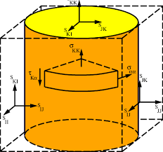
物理代写|广义相对论代写General relativity代考|Tetrads and n-Trads
In general relativity we often find it useful to use tetrads, a set of four basis vectors that forms an orthonormal basis as in special relativity. This sets up a reference frame at a point that is analogous to the reference frame of special relativity. The tetrad differs from the set of coordinate basis vectors in that it is normalized and need not align with the coordinate axes. More generally, in $n$ dimensions we define an $n$-trad, a set of $n$ basis vectors $\vec{e}{a}$ oriented and normalized so that $$ \vec{e}{a} \cdot \vec{e}{b}=\eta{a b}
$$
where the $\eta_{a b}$ matrix is chosen for convenience. It is usually taken to be the constant Lorentz metric in relativity theory but may be any constant matrix such as the Kronecker delta as needed in other situations; we refer to it as the $n$-trad metric. In this section the $n$-trads will be labeled with lower Latin indices early in the alphabet like $b$, and the space indices will usually be Greek.
Notice that the local Lorentz frame we previously discussed is essentially the same as the frame provided by the tetrads. Indeed it is possible to develop the theory of tetrads based on the transformation to the local Lorentz frame, although we will not do that here (Lawrie 1990).
In this section we will denote the coordinate basis as $\vec{g}{\beta}$ to distinguish it from the $n$-trad basis $\vec{e}{a}$, and it will be labeled with Greek indices. The $n$-trad may be expanded in terms of the coordinate basis as
$$
\vec{e}{a}=e{a}^{\beta} \vec{g}{\beta}, \quad e{a}^{\beta}=n \text {-trad components in coordinate basis. }
$$
This gives a beautiful relation for the $n$-trad metric in terms of the metric,
$$
\begin{aligned}
&\eta_{a b}=\vec{e}{a} \cdot \vec{e}{b}=\left(e_{a}^{\beta} \vec{g}{\beta}\right) \cdot\left(e{b}^{\mu} \vec{g}{\mu}\right)=e{a}^{\beta} e_{b}^{\mu}\left(\vec{g}{\beta} \cdot \vec{g}{\mu}\right)=e_{a}^{\beta} e_{b}^{\mu} g_{\beta \mu}, \
&\eta_{a b}=e_{a}^{\beta} e_{b}^{\mu} g_{\beta \mu}
\end{aligned}
$$
广义相对论代考
物理代写|广义相对论代写General relativity代考|Tensors, Component View
在本节中,我们继续使用向量和张量作为索引数组的经典组件视图。本节主要由一组定理组成,这些定理通过通常称为索引杂耍的相对简单的代数过程证明。应该清楚的是,经过一些练习,指标的平衡为我们做了很多工作。
为了定义张量,我们将向量的概念概括为定义为n-在坐标系之间具有明确转换的元组:张量被定义为一组具有任意数量索引的量,其转换根据
吨¯米…l…=∂X¯l∂Xq…∂Xn∂X¯米…吨q……, 张量分量。 指数的总数称为排名;一些指数可能较高或逆变,而其他指数可能较低或协变。此类索引的数量写为(米,ñ). 因此,例如,向量是一阶张量和 (1, 0 )。另一个例子是在j在q,这是一个二阶张量和(1,1).
从这个张量定义中可以得出许多简单但强大的定理。我们已经在 Sect 中介绍并证明了其中的两个。4.2:定理1涉及雅可比矩阵,定理2涉及向量内积的不变性。让我们继续讨论更多这样的定理。
定理 3 为了收缩一个张量,我们设置一个上限指数等于一个下限指数和总和,这给出了另一个张量;例如一个收缩吨一个bλ是是吨bC一个b=小号一个C. 秩的收缩r张量产生等级r−2张量。以上述 4 阶张量为例。然后收缩对象变换为吨¯bC一个b=∂X¯一个∂Xω∂X¯b∂Xσ∂Xλ∂X¯b∂X这∂X¯C吨ωσλ这=∂X¯一个∂Xωdσλ∂X这∂X¯C吨ωωσλ这∂X这 =∂X¯一个∂Xωω∂X这∂X¯C吨σ这ωω.
物理代写|广义相对论代写General relativity代考|Tensors, Abstract View
与向量一样,我们可以将张量视为抽象对象,而不是从上一节讨论的经典组件的角度来看。在这种抽象方法中,(米,ñ)张量被定义为线性映射米向量和ñ-形式到实数。例如一个(0,2)张量吨用作向量上的线性映射在→,在→如下
吨(在→,在→)=吨(在b和→b,在μ和→μ)=在b在μ吨(和→b,和→μ)≡在b在μ吨bμ
组件吨bμ这里定义的与我们在上一节中讨论的相同。因此一个向量也是一个(1,0)张量和 1 形式也是(0,1)张量。度量是最重要的特例(0,2)张量,所以我们明确地注意到它在组件方面的操作
G(在→,在→)=在b在μGbμ
让我们看另一个例子(0,2)张量。将两个 1 形式的直接乘积定义为在两个向量上线性运算以通过以下自然方式给出实数的东西,
p~⊗q~= 1-形式的直接乘积, p~⊗q~(在→,在→)=p~(在→)q~(在→)
也就是说,直积中的第一个因子对第一个向量进行运算,而直接积中的第二个因子对第二个向量进行运算。因此 (4.56) 中的直积是(0,2)张量。应该清楚的是,我们可以将定义扩展到任意数的直积米的 1 形状因子以产生(0,米)张量等等。
回想一下我们在 Sect 中讨论过的内容。4.31-形式的基础,我们表示为ω~一个. 我们可以类似地证明存在两个 1 形式或 ( 0 , 2) 张量的乘积的基础。实际上,基础是直接乘积的线性组合ω~一个. 我们将该线性组合写为
F=F一个bω~一个⊗ω~b.
物理代写|广义相对论代写General relativity代考|Tetrads and n-Trads
在广义相对论中,我们经常发现使用四分体很有用,四分体是一组四个基向量,形成一个正交基,就像狭义相对论中一样。这在类似于狭义相对论的参考系的点上建立了一个参考系。四分体与坐标基向量集的不同之处在于它是标准化的并且不需要与坐标轴对齐。更一般地,在n我们定义的维度n-trad,一组n基向量和→一个定向和规范化,使得
和→一个⋅和→b=这一个b
在哪里这一个b为方便起见选择矩阵。它通常被认为是相对论中的常数 Lorentz 度量,但在其他情况下也可以是任何常数矩阵,例如 Kronecker delta;我们将其称为n-传统指标。在本节中n-trads 将在字母表的开头标有较低的拉丁索引,例如b,并且空间索引通常是希腊语。
请注意,我们之前讨论的局部洛伦兹框架与四分体提供的框架基本相同。实际上,有可能基于局部洛伦兹框架的变换来发展四分体理论,尽管我们不会在这里这样做(Lawrie 1990)。
在本节中,我们将坐标基表示为G→b将其与n- 贸易基础和→一个, 它将用希腊索引标记。这n-trad 可以在坐标基础上扩展为
和→一个=和一个bG→b,和一个b=n-在坐标基础上的传统组件。
这为n- 就度量而言的传统度量,
这一个b=和→一个⋅和→b=(和一个bG→b)⋅(和bμG→μ)=和一个b和bμ(G→b⋅G→μ)=和一个b和bμGbμ, 这一个b=和一个b和bμGbμ

统计代写请认准statistics-lab™. statistics-lab™为您的留学生涯保驾护航。
金融工程代写
金融工程是使用数学技术来解决金融问题。金融工程使用计算机科学、统计学、经济学和应用数学领域的工具和知识来解决当前的金融问题,以及设计新的和创新的金融产品。
非参数统计代写
非参数统计指的是一种统计方法,其中不假设数据来自于由少数参数决定的规定模型;这种模型的例子包括正态分布模型和线性回归模型。
广义线性模型代考
广义线性模型(GLM)归属统计学领域,是一种应用灵活的线性回归模型。该模型允许因变量的偏差分布有除了正态分布之外的其它分布。
术语 广义线性模型(GLM)通常是指给定连续和/或分类预测因素的连续响应变量的常规线性回归模型。它包括多元线性回归,以及方差分析和方差分析(仅含固定效应)。
有限元方法代写
有限元方法(FEM)是一种流行的方法,用于数值解决工程和数学建模中出现的微分方程。典型的问题领域包括结构分析、传热、流体流动、质量运输和电磁势等传统领域。
有限元是一种通用的数值方法,用于解决两个或三个空间变量的偏微分方程(即一些边界值问题)。为了解决一个问题,有限元将一个大系统细分为更小、更简单的部分,称为有限元。这是通过在空间维度上的特定空间离散化来实现的,它是通过构建对象的网格来实现的:用于求解的数值域,它有有限数量的点。边界值问题的有限元方法表述最终导致一个代数方程组。该方法在域上对未知函数进行逼近。[1] 然后将模拟这些有限元的简单方程组合成一个更大的方程系统,以模拟整个问题。然后,有限元通过变化微积分使相关的误差函数最小化来逼近一个解决方案。
tatistics-lab作为专业的留学生服务机构,多年来已为美国、英国、加拿大、澳洲等留学热门地的学生提供专业的学术服务,包括但不限于Essay代写,Assignment代写,Dissertation代写,Report代写,小组作业代写,Proposal代写,Paper代写,Presentation代写,计算机作业代写,论文修改和润色,网课代做,exam代考等等。写作范围涵盖高中,本科,研究生等海外留学全阶段,辐射金融,经济学,会计学,审计学,管理学等全球99%专业科目。写作团队既有专业英语母语作者,也有海外名校硕博留学生,每位写作老师都拥有过硬的语言能力,专业的学科背景和学术写作经验。我们承诺100%原创,100%专业,100%准时,100%满意。
随机分析代写
随机微积分是数学的一个分支,对随机过程进行操作。它允许为随机过程的积分定义一个关于随机过程的一致的积分理论。这个领域是由日本数学家伊藤清在第二次世界大战期间创建并开始的。
时间序列分析代写
随机过程,是依赖于参数的一组随机变量的全体,参数通常是时间。 随机变量是随机现象的数量表现,其时间序列是一组按照时间发生先后顺序进行排列的数据点序列。通常一组时间序列的时间间隔为一恒定值(如1秒,5分钟,12小时,7天,1年),因此时间序列可以作为离散时间数据进行分析处理。研究时间序列数据的意义在于现实中,往往需要研究某个事物其随时间发展变化的规律。这就需要通过研究该事物过去发展的历史记录,以得到其自身发展的规律。
回归分析代写
多元回归分析渐进(Multiple Regression Analysis Asymptotics)属于计量经济学领域,主要是一种数学上的统计分析方法,可以分析复杂情况下各影响因素的数学关系,在自然科学、社会和经济学等多个领域内应用广泛。
MATLAB代写
MATLAB 是一种用于技术计算的高性能语言。它将计算、可视化和编程集成在一个易于使用的环境中,其中问题和解决方案以熟悉的数学符号表示。典型用途包括:数学和计算算法开发建模、仿真和原型制作数据分析、探索和可视化科学和工程图形应用程序开发,包括图形用户界面构建MATLAB 是一个交互式系统,其基本数据元素是一个不需要维度的数组。这使您可以解决许多技术计算问题,尤其是那些具有矩阵和向量公式的问题,而只需用 C 或 Fortran 等标量非交互式语言编写程序所需的时间的一小部分。MATLAB 名称代表矩阵实验室。MATLAB 最初的编写目的是提供对由 LINPACK 和 EISPACK 项目开发的矩阵软件的轻松访问,这两个项目共同代表了矩阵计算软件的最新技术。MATLAB 经过多年的发展,得到了许多用户的投入。在大学环境中,它是数学、工程和科学入门和高级课程的标准教学工具。在工业领域,MATLAB 是高效研究、开发和分析的首选工具。MATLAB 具有一系列称为工具箱的特定于应用程序的解决方案。对于大多数 MATLAB 用户来说非常重要,工具箱允许您学习和应用专业技术。工具箱是 MATLAB 函数(M 文件)的综合集合,可扩展 MATLAB 环境以解决特定类别的问题。可用工具箱的领域包括信号处理、控制系统、神经网络、模糊逻辑、小波、仿真等。