如果你也在 怎样代写理论力学theoretical mechanics这个学科遇到相关的难题,请随时右上角联系我们的24/7代写客服。
理论力学主要研究物体的力学性能及运动规律,是力学的基础学科,由静力学、运动学和动力学三大部分组成。也有人认为运动学是动力学的一部分,而提出二分法。
statistics-lab™ 为您的留学生涯保驾护航 在代写理论力学theoretical mechanics方面已经树立了自己的口碑, 保证靠谱, 高质且原创的统计Statistics代写服务。我们的专家在代写理论力学theoretical mechanics代写方面经验极为丰富,各种代写理论力学theoretical mechanics相关的作业也就用不着说。
我们提供的理论力学theoretical mechanics及其相关学科的代写,服务范围广, 其中包括但不限于:
- Statistical Inference 统计推断
- Statistical Computing 统计计算
- Advanced Probability Theory 高等概率论
- Advanced Mathematical Statistics 高等数理统计学
- (Generalized) Linear Models 广义线性模型
- Statistical Machine Learning 统计机器学习
- Longitudinal Data Analysis 纵向数据分析
- Foundations of Data Science 数据科学基础
物理代写|理论力学代写theoretical mechanics代考|Infinite Periodic System. Plane Problem
The solution to the plane elasticity theory for the infinite periodic systems by the developed semi-analytical method is presented in $[16,17]$. Let us cite here only the properties of the kernel for respective integral equations and the discretization scheme.
As indicated above, it is necessary to consider the auxiliary integral equation, for which we should study the properties of its kernel $[16,17]$ :
$$
\begin{aligned}
&\frac{1}{2 a} \int_{-b}^{b} h(\eta) K(y-\eta) d \eta=1 ; K(y)=\sum_{n=1}^{\infty} L_{n} \cos \left(a_{n} y\right) ; L_{n}=\frac{R_{n}}{k_{2}^{2} q_{n}},|y|<b \
&q_{n}=\left[(\pi n / a)^{2}-k_{1}^{2}\right]^{1 / 2}, r_{n}=\left[(\pi n / a)^{2}-k_{2}^{2}\right]^{1 / 2},
\end{aligned}
$$
$$
R_{n}=\left[2 a_{n}^{2}-k_{2}^{2}\right]^{2}-4 r_{n} q_{n} a_{n}^{2}, \quad a_{n}=\pi n / a
$$
Here $k_{1}, k_{2}$-wave numbers for the longitudinal and the transverse waves. Let us notice that $L_{n} \sim-2\left(1-c_{2}^{2} / c_{1}^{2}\right) a_{n}, n \rightarrow \infty$, where $c_{1}, c_{2}$-the speed of the longitudinal and the transverse wave, respectively. Then the expression for the kernel is transformed to the following form
$$
\begin{aligned}
K(y) &=-2\left(1-\frac{c_{2}^{2}}{c_{1}^{2}}\right) \sum_{n=1}^{\infty} a_{n} \cos \left(a_{n} y\right)+\sum_{n=1}^{\infty}\left[L_{n}+2\left(1-\frac{c_{2}^{2}}{c_{1}^{2}}\right) a_{n}\right] \cos \left(a_{n} y\right) \
&=-2\left(1-\frac{c_{2}^{2}}{c_{1}^{2}}\right) I(y)+K_{r}(y)
\end{aligned}
$$
Here the second sum is a certain regular function. The first one has both regular and singular parts: $I(y)=\left[I_{r}(y)+I_{s}(y)\right]$. After some transformations of the kernel (15) of the auxiliary integral Eq. (14) the regular and the singular parts become, respectively
$$
I_{r}(y)=\frac{a}{\pi y^{2}}-\frac{\pi}{4 a \sin ^{2}(\pi y / 2 a)} ; I_{s}(y)=-\frac{a}{\pi y^{2}}
$$
物理代写|理论力学代写theoretical mechanics代考|Finite Periodic System. Scalar Formulation
In order to solve the problem in the scalar case, we first consider the incidence of a plane wave upon a doubly-periodic system of rigid screens, which is finite in the both directions. In frames of the scalar acoustics, the wave equation for full acoustic pressure $p$ is reduced to the Helmholtz equation
$$
\left(\Delta+k^{2}\right) \mathbf{p}=0
$$
where $k$-the wave number of the acoustic wave, $\Delta$ denotes the two-dimensional Laplace operator, and the full wave pressure is a linear sum of the incident and the scattered field: $\mathbf{p}=\mathbf{p}^{i n c}+\mathbf{p}^{s c}$. To be more specific, let us restrict the consideration by the normal incidence of a plane wave, hence the incident wave field is $\mathbf{p}^{i n c}\left(y^{0}\right)=$ $\mathrm{e}^{i k y_{1}^{0}}$, where the two-dimensional point is $y^{0}=\left(y_{1}^{0}, y_{2}^{0}\right)$.
The boundary condition, in the case of acoustically hard boundary $\bar{L}$ has the form
$$
\left.\frac{\partial \mathbf{p}}{\partial \mathbf{n}{y}}\right|{\tilde{L}}=0, \quad(y \in \tilde{L})
$$
Here $\mathbf{n}{y}$ is the unit normal vector at the point $y$, and $\bar{L}=\sum{m=1}^{M} \tilde{l}_{m}$ represents itself the full set of boundary contours.
In order to develop the basic boundary integral equation, let us introduce a respective closed contour $l_{m}$ around the current screen. Obviously, for the given contours, in the case when the observation point $x$ is outside, the following standard integral representation is valid
$$
p^{s c}\left(y^{0}\right)=\int_{L}\left(p(y) \frac{\partial \Phi}{\partial n_{y}}-\frac{\partial p(y)}{\partial n_{y}} \Phi\right) d L_{y}, \quad(y \in L)
$$
where $\Phi=\Phi(r)$ is the Green’s function, which in the two-dimensional acoustic case is expressed through the Hankel function of the first kind $\Phi(r)=(i / 4) H_{0}^{(1)}(r), r=$ $\left|y-y^{0}\right|$
If each surrounding closed contour converges to the respective rigid screen located inside, then the second term in $(22)$ is cancelled, due to the boundary condition. The opposite sides of each obstacle are considered separately, being $l_{m}^{-}$и $l_{m}^{+}$, where the sign “plus” is related to the normal $\mathbf{n}{m}^{+}$, directed along the propagation of the incident wave, and the negative sign-oppositely. Then, the integral representation (22) can be reduced to the expression $$ \begin{aligned} \mathbf{p}^{s c}\left(y^{0}\right) &=\sum{m=1}^{M}\left(\int_{\ell_{w}^{+}}\left(\mathbf{p}^{+}(y) \frac{\partial \Phi}{\partial \mathbf{n}{y}^{+}}\right) d \ell{y}^{+}+\int\left(\mathbf{p}^{-}(y) \frac{\partial \Phi}{\partial \mathbf{n}{y}^{-}}\right) d \ell{y}^{-}\right) \
&=\sum_{m=1}^{M} \int_{\ell_{m}^{+}} \mathbf{g}(y) \frac{\partial \Phi}{\partial \mathbf{n}{y}^{+}}\left(k\left|y-y^{0}\right|\right) d \ell{y}^{+}, \mathbf{g}(y)=\mathbf{p}^{+}(y)-\mathbf{p}^{-}(y), \quad\left(y \in l_{m}\right)
\end{aligned}
$$
物理代写|理论力学代写theoretical mechanics代考|Numerical Analysis
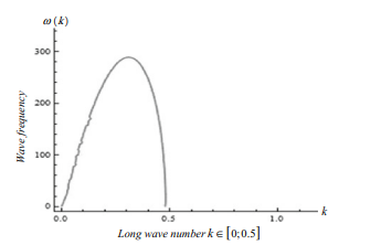
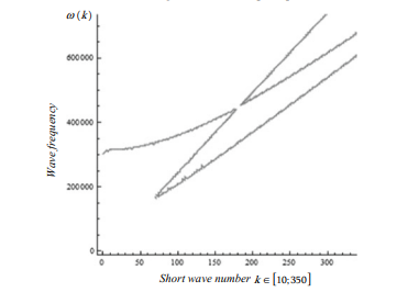
Let us perform a numerical analysis of the problems considered above, on example of the medium with the longitudinal wave speed $c_{1}=6000 \mathrm{~m} / \mathrm{s}$ (steel), and the ratio of the longitudinal and the transverse wave speeds is $c_{1} / c_{2}=1.87$.
To begin with, let us compare the moduli of reflection and transmission coefficients versus frequency parameter, between the three studied cases, for a single vertical array (see Figs. 2 and 3). With so doing, we assume that the longitudinal wave speed in the problem 2 is equal to the transverse wave speed of the problems 1 and 3. This condition shortens the one-mode frequency interval, whose limit from the right becomes $\pi / 1.87=1.680$, (see Figs. 2 and 3 ). In Figs. $4,5,6,7$ and 8 the comparative numerical analysis of the scalar problems 1 and 3 has been performed for the transverse incident wave. Let us notice that for all cases the filtration interval can be seen in the upper part of the one-mode frequency range. It is shown that lines 2 and 3 in Figs. 2 and 3, related to the scalar problems, are practically coinciding that takes place even for $N=10$ cracks in each vertical array. It should also be noted that line 1 related to the elastic problem, shows a significant domination of the filtration property, when compared with both infinite and finite scalar problems. Let us also notice that for two vertical arrays in the elastic problem a perfect filtration takes place for $a k \geq 0.7$, but for one vertical row this property is valid only for $a k \geq 1.5$; this also confirms the evident property that with the growth of the vertical rows the filtration becomes stronger.
Let us pass to the analysis of the grid size to the precision of the obtained results. It is stated that in the case of a single obstacle it is sufficient to take 10 grid nodes per each wavelength, to provide reliable results. With so doing, for the frequency $0.16 \mathrm{MHz}$ in this formulation the wavelength is $3.75 \mathrm{~cm}$, hence on the obstacle of the length $1.5 \mathrm{~cm}$ it is sufficient to take only 5 nodes. However, the complex geometry of the diffraction lattice requires greater number of nodes. It can be seen from Fig. 4 , which represents the results for the array of 10 vertical rows, each containing 10 obstacles, that with 10 nodes over each obstacle the calculations are correct only in the low-frequency case (for $k^{*} a<1$ ).
理论力学代考
物理代写|理论力学代写theoretical mechanics代考|Infinite Periodic System. Plane Problem
用发达的半解析方法求解无限周期系统的平面弹性理论[16,17]. 让我们在这里仅引用各个积分方程和离散化方案的核的属性。
如上所述,有必要考虑辅助积分方程,为此我们应该研究其核的性质[16,17] :
12一个∫−bbH(这)ķ(是−这)d这=1;ķ(是)=∑n=1∞大号n因(一个n是);大号n=Rnķ22qn,|是|<b qn=[(圆周率n/一个)2−ķ12]1/2,rn=[(圆周率n/一个)2−ķ22]1/2,
Rn=[2一个n2−ķ22]2−4rnqn一个n2,一个n=圆周率n/一个
这里ķ1,ķ2- 纵波和横波的波数。让我们注意到大号n∼−2(1−C22/C12)一个n,n→∞, 在哪里C1,C2- 分别为纵波和横波的速度。然后内核的表达式转换为以下形式
ķ(是)=−2(1−C22C12)∑n=1∞一个n因(一个n是)+∑n=1∞[大号n+2(1−C22C12)一个n]因(一个n是) =−2(1−C22C12)我(是)+ķr(是)
这里的第二个和是某个正则函数。第一个有常规部分和奇异部分:我(是)=[我r(是)+我s(是)]. 经过辅助积分方程的核(15)的一些变换。(14) 正则部分和奇异部分分别变为
我r(是)=一个圆周率是2−圆周率4一个罪2(圆周率是/2一个);我s(是)=−一个圆周率是2
物理代写|理论力学代写theoretical mechanics代考|Finite Periodic System. Scalar Formulation
为了解决标量情况下的问题,我们首先考虑平面波在刚性屏幕的双周期系统上的入射,该系统在两个方向上都是有限的。在标量声学框架中,全声压的波动方程p简化为亥姆霍兹方程
(Δ+ķ2)p=0
在哪里ķ-声波的波数,Δ表示二维拉普拉斯算子,全波压力是入射场和散射场的线性和:p=p一世nC+psC. 更具体地说,让我们通过平面波的垂直入射来限制考虑,因此入射波场是p一世nC(是0)= 和一世ķ是10,其中二维点为是0=(是10,是20).
边界条件,在声学硬边界的情况下大号¯有形式
∂p∂n是|大号~=0,(是∈大号~)
这里n是是该点的单位法向量是, 和大号¯=∑米=1米l~米代表自己完整的边界轮廓集。
为了发展基本的边界积分方程,让我们引入一个各自的闭合轮廓l米在当前屏幕周围。显然,对于给定的轮廓,当观察点X在外面,下面的标准积分表示是有效的
psC(是0)=∫大号(p(是)∂披∂n是−∂p(是)∂n是披)d大号是,(是∈大号)
在哪里披=披(r)是格林函数,在二维声学情况下通过第一类汉克尔函数表示披(r)=(一世/4)H0(1)(r),r= |是−是0|
如果每个周围的闭合轮廓都收敛到位于内部的相应刚性屏幕,则第二项(22)由于边界条件,被取消。分别考虑每个障碍物的相对侧,即l米−一世l米+,其中符号“加号”与法线有关n米+,沿着入射波的传播方向,负号相反。然后,积分表示(22)可以简化为表达式
psC(是0)=∑米=1米(∫ℓ在+(p+(是)∂披∂n是+)dℓ是++∫(p−(是)∂披∂n是−)dℓ是−) =∑米=1米∫ℓ米+G(是)∂披∂n是+(ķ|是−是0|)dℓ是+,G(是)=p+(是)−p−(是),(是∈l米)
物理代写|理论力学代写theoretical mechanics代考|Numerical Analysis
让我们对上面考虑的问题进行数值分析,以具有纵波速度的介质为例C1=6000 米/s(钢),纵波和横波速度之比为C1/C2=1.87.
首先,让我们比较三个研究案例中单个垂直阵列的反射和透射系数的模量与频率参数的关系(见图 2 和图 3)。这样做,我们假设问题 2 中的纵波速度等于问题 1 和问题 3 的横波速度。这个条件缩短了单模频率间隔,其从右边的极限变为圆周率/1.87=1.680, (见图 2 和 3)。在无花果。4,5,6,7图 8 对横向入射波进行了标量问题 1 和 3 的比较数值分析。让我们注意到,对于所有情况,过滤间隔都可以在单模频率范围的上部看到。可以看出,图 2 和 3 中的第 2 行和第 3 行。与标量问题相关的 2 和 3 实际上是重合的,即使对于ñ=10每个垂直阵列中的裂缝。还应该注意的是,与无限和有限标量问题相比,与弹性问题相关的第 1 行显示了过滤特性的显着优势。让我们也注意到,对于弹性问题中的两个垂直阵列,一个完美的过滤发生在一个ķ≥0.7,但对于一个垂直行,此属性仅对一个ķ≥1.5; 这也证实了随着垂直行的增长过滤变得更强的明显特性。
让我们通过对网格大小的分析来获得结果的精度。据称,在单个障碍物的情况下,每个波长采用 10 个网格节点就足以提供可靠的结果。这样做,对于频率0.16米H和在这个公式中,波长是3.75 C米,因此在长度的障碍上1.5 C米只需要 5 个节点就足够了。然而,衍射晶格的复杂几何形状需要更多的节点。从图 4 可以看出,它表示 10 个垂直行的阵列的结果,每行包含 10 个障碍物,每个障碍物上有 10 个节点,计算仅在低频情况下是正确的(对于ķ∗一个<1 ).

统计代写请认准statistics-lab™. statistics-lab™为您的留学生涯保驾护航。
金融工程代写
金融工程是使用数学技术来解决金融问题。金融工程使用计算机科学、统计学、经济学和应用数学领域的工具和知识来解决当前的金融问题,以及设计新的和创新的金融产品。
非参数统计代写
非参数统计指的是一种统计方法,其中不假设数据来自于由少数参数决定的规定模型;这种模型的例子包括正态分布模型和线性回归模型。
广义线性模型代考
广义线性模型(GLM)归属统计学领域,是一种应用灵活的线性回归模型。该模型允许因变量的偏差分布有除了正态分布之外的其它分布。
术语 广义线性模型(GLM)通常是指给定连续和/或分类预测因素的连续响应变量的常规线性回归模型。它包括多元线性回归,以及方差分析和方差分析(仅含固定效应)。
有限元方法代写
有限元方法(FEM)是一种流行的方法,用于数值解决工程和数学建模中出现的微分方程。典型的问题领域包括结构分析、传热、流体流动、质量运输和电磁势等传统领域。
有限元是一种通用的数值方法,用于解决两个或三个空间变量的偏微分方程(即一些边界值问题)。为了解决一个问题,有限元将一个大系统细分为更小、更简单的部分,称为有限元。这是通过在空间维度上的特定空间离散化来实现的,它是通过构建对象的网格来实现的:用于求解的数值域,它有有限数量的点。边界值问题的有限元方法表述最终导致一个代数方程组。该方法在域上对未知函数进行逼近。[1] 然后将模拟这些有限元的简单方程组合成一个更大的方程系统,以模拟整个问题。然后,有限元通过变化微积分使相关的误差函数最小化来逼近一个解决方案。
tatistics-lab作为专业的留学生服务机构,多年来已为美国、英国、加拿大、澳洲等留学热门地的学生提供专业的学术服务,包括但不限于Essay代写,Assignment代写,Dissertation代写,Report代写,小组作业代写,Proposal代写,Paper代写,Presentation代写,计算机作业代写,论文修改和润色,网课代做,exam代考等等。写作范围涵盖高中,本科,研究生等海外留学全阶段,辐射金融,经济学,会计学,审计学,管理学等全球99%专业科目。写作团队既有专业英语母语作者,也有海外名校硕博留学生,每位写作老师都拥有过硬的语言能力,专业的学科背景和学术写作经验。我们承诺100%原创,100%专业,100%准时,100%满意。
随机分析代写
随机微积分是数学的一个分支,对随机过程进行操作。它允许为随机过程的积分定义一个关于随机过程的一致的积分理论。这个领域是由日本数学家伊藤清在第二次世界大战期间创建并开始的。
时间序列分析代写
随机过程,是依赖于参数的一组随机变量的全体,参数通常是时间。 随机变量是随机现象的数量表现,其时间序列是一组按照时间发生先后顺序进行排列的数据点序列。通常一组时间序列的时间间隔为一恒定值(如1秒,5分钟,12小时,7天,1年),因此时间序列可以作为离散时间数据进行分析处理。研究时间序列数据的意义在于现实中,往往需要研究某个事物其随时间发展变化的规律。这就需要通过研究该事物过去发展的历史记录,以得到其自身发展的规律。
回归分析代写
多元回归分析渐进(Multiple Regression Analysis Asymptotics)属于计量经济学领域,主要是一种数学上的统计分析方法,可以分析复杂情况下各影响因素的数学关系,在自然科学、社会和经济学等多个领域内应用广泛。
MATLAB代写
MATLAB 是一种用于技术计算的高性能语言。它将计算、可视化和编程集成在一个易于使用的环境中,其中问题和解决方案以熟悉的数学符号表示。典型用途包括:数学和计算算法开发建模、仿真和原型制作数据分析、探索和可视化科学和工程图形应用程序开发,包括图形用户界面构建MATLAB 是一个交互式系统,其基本数据元素是一个不需要维度的数组。这使您可以解决许多技术计算问题,尤其是那些具有矩阵和向量公式的问题,而只需用 C 或 Fortran 等标量非交互式语言编写程序所需的时间的一小部分。MATLAB 名称代表矩阵实验室。MATLAB 最初的编写目的是提供对由 LINPACK 和 EISPACK 项目开发的矩阵软件的轻松访问,这两个项目共同代表了矩阵计算软件的最新技术。MATLAB 经过多年的发展,得到了许多用户的投入。在大学环境中,它是数学、工程和科学入门和高级课程的标准教学工具。在工业领域,MATLAB 是高效研究、开发和分析的首选工具。MATLAB 具有一系列称为工具箱的特定于应用程序的解决方案。对于大多数 MATLAB 用户来说非常重要,工具箱允许您学习和应用专业技术。工具箱是 MATLAB 函数(M 文件)的综合集合,可扩展 MATLAB 环境以解决特定类别的问题。可用工具箱的领域包括信号处理、控制系统、神经网络、模糊逻辑、小波、仿真等。