如果你也在 怎样代写理论力学theoretical mechanics这个学科遇到相关的难题,请随时右上角联系我们的24/7代写客服。
理论力学主要研究物体的力学性能及运动规律,是力学的基础学科,由静力学、运动学和动力学三大部分组成。也有人认为运动学是动力学的一部分,而提出二分法。
statistics-lab™ 为您的留学生涯保驾护航 在代写理论力学theoretical mechanics方面已经树立了自己的口碑, 保证靠谱, 高质且原创的统计Statistics代写服务。我们的专家在代写理论力学theoretical mechanics代写方面经验极为丰富,各种代写理论力学theoretical mechanics相关的作业也就用不着说。
我们提供的理论力学theoretical mechanics及其相关学科的代写,服务范围广, 其中包括但不限于:
- Statistical Inference 统计推断
- Statistical Computing 统计计算
- Advanced Probability Theory 高等概率论
- Advanced Mathematical Statistics 高等数理统计学
- (Generalized) Linear Models 广义线性模型
- Statistical Machine Learning 统计机器学习
- Longitudinal Data Analysis 纵向数据分析
- Foundations of Data Science 数据科学基础
物理代写|理论力学代写theoretical mechanics代考|Space and Time
Space and time are two basic concepts which, according to Kant, inherently or innately determine the form of all experience in an a priori manner, thereby making possible experience as such: only in space and time can we arrange our sensations. [According to the doctrines of evolutionary cognition, what is innate to us has developed phylogenetically by adaption to our environment. This is why we only notice the insufficiency of these “self-evident”‘ concepts under extraordinary circumstances, e.g., for velocities close to that of light $\left(c_{0}\right)$ or actions of the order of Planck’s quantum $h$. We shall tackle such “weird” cases later-in electromagnetism and quantum mechanics. For the time being, we want to make sure we can handle our familiar environment.]
To do this, we introduce a continuous parameter $t$. Like every other physical quantity it is composed of number and unit (for example, a second $1 \mathrm{~s}=1 \mathrm{~min} / 60$ $-1 \mathrm{~h} / 3600$ ). The larger the unit, the smaller the number. Physical quantities do not depend on the unit-likewise equations between physical quantities. Nevertheless, the opposite is sometimes seen, as in: “We choose units such that the velocity of light $c$ assumes the value 1”. In fact, the concept of velocity is thereby changed, so that instead of the velocity $v$, the ratio $v / c$ is taken here as the velocity, and $c t$ as time or $x / c$ as length.
The zero time $(t=0)$ can be chosen arbitrarily, since basically only the time difference, i.e., the duration of a process, is important. A differentiation with respect to time $(\mathrm{d} / \mathrm{d} t)$ is often marked by a dot over the differentiated quantity, i.e., $\mathrm{d} x / \mathrm{d} t \equiv \dot{x}$.
In empty space every direction is equivalent. Here, too, we may choose the zero point freely and, starting from this point, determine the position of other points in a coordinate-free notation by the position vector $\mathbf{r}$, which fixes the distance and direction of the point under consideration. This coordinate-free type of notation is particularly advantageous when we want to exploit the assumed homogeneity of space. However, conditions often arise (i.e., when there is axial or spherical symmetry) which are best taken care of in special coordinates. We are free to choose a coordinate system. We only require that it determine all positions uniquely. This we shall treat in the next section.
物理代写|理论力学代写theoretical mechanics代考|Vector Algebra
From two vectors $\mathbf{a}$ and $\mathbf{b}$, their sum $\mathbf{a}+\mathbf{b}$ may be formed according to the construction of parallelograms (as the diagonal), as shown in Fig. 1.1. From this follows the commutative and associative law of vector addition:
$$
\mathbf{a}+\mathbf{b}=\mathbf{b}+\mathbf{a}, \quad(\mathbf{a}+\mathbf{b})+\mathbf{c}=\mathbf{a}+(\mathbf{b}+\mathbf{c})
$$
The product of the vectors a with a scalar (i.e., directionless) factor $\alpha$ is understood as the vector $\alpha \mathbf{a}=\mathbf{a} \alpha$ with the same (for $\alpha<0$ opposite) direction and with value $|\alpha| a$. In particular, a and $-\mathbf{a}$ have the same value, but opposite directions. For $\alpha=0$ the zero vector 0 results, with length 0 and undetermined direction.
The scalar product (inner product) $\mathbf{a} \cdot \mathbf{b}$ of the two vectors $\mathbf{a}$ and $\mathbf{b}$ is the product of their values times the cosine of the enclosed angle $\phi_{a b}$ (see Fig. 1.2 left):
$$
\mathbf{a} \cdot \mathbf{b} \equiv a b \cos \phi_{a b}
$$
The dot between the two factors is important for the scalar product-if it is missing, then it is the tensor product of the two vectors, which will be explained in Sect. 1.2.4 with $\mathbf{a} \cdot \mathbf{b} \mathbf{c} \neq \mathbf{a} \mathbf{b} \cdot \mathbf{c}$, if $\mathbf{a}$ and $\mathbf{c}$ have different directions, i.e., if $\mathbf{a}$ is not a multiple of $\mathbf{c}$. Consequently, one has
$$
\mathbf{a} \cdot \mathbf{b}=\mathbf{b} \cdot \mathbf{a}
$$
and
$$
\mathbf{a} \cdot \mathbf{b}=0 \quad \Longleftrightarrow \quad \mathbf{a} \perp \mathbf{b} \text { or } a=0 \text { or } b=0 .
$$
If the two vectors are oriented perpendicularly to each other $(\mathbf{a} \perp \mathbf{b})$, then they are also said to be orthogonal. Obviously, $\mathbf{a} \cdot \mathbf{a}=a^{2}$ holds. Vectors with value 1 are called unit vectors. Here they are denoted by e. Given three Cartesian, i.e., pairwise perpendicular unit vectors $\mathbf{e}{x}, \mathbf{e}{y}, \mathbf{e}{z}$, all vectors can be decomposed in terms of these: $$ \mathbf{a}=\mathbf{e}{x} a_{x}+\mathbf{e}{y} a{y}+\mathbf{e}{z} a{z},
$$
with the Cartesian components
$$
a_{x} \equiv \mathbf{e}{x} \cdot \mathbf{a}, \quad a{y} \equiv \mathbf{e}{y} \cdot \mathbf{a}, \quad a{z} \equiv \mathbf{e}_{z} \cdot \mathbf{a} .
$$
物理代写|理论力学代写theoretical mechanics代考|Trajectories
If a vector depends upon a parameter, then we speak of a vector function. The vector function $\mathbf{a}(t)$ is continuous at $t_{0}$, if it tends to $\mathbf{a}\left(t_{0}\right)$ for $t \rightarrow t_{0}$. With the same limit $t \rightarrow t_{0}$, the vector differential da and the first derivative da/d $t$ is introduced. These quantities may be formed for every Cartesian component, and we have
$$
\begin{array}{ll}
\mathrm{d}(\mathbf{a}+\mathbf{b})=\mathrm{d} \mathbf{a}+\mathrm{d} \mathbf{b}, & \mathrm{d}(\alpha \mathbf{a})=\alpha \mathrm{d} \mathbf{a}+\mathbf{a} \mathrm{d} \alpha \
\mathrm{d}(\mathbf{a} \cdot \mathbf{b})=\mathbf{a} \cdot \mathrm{d} \mathbf{b}+\mathbf{b} \cdot \mathrm{d} \mathbf{a}, & \mathrm{d}(\mathbf{a} \times \mathbf{b})=\mathbf{a} \times \mathrm{d} \mathbf{b}-\mathbf{b} \times \mathrm{d} \mathbf{a}
\end{array}
$$
Obviously, $\mathbf{a} \cdot \mathrm{d} \mathbf{a} / \mathrm{d} t=\frac{1}{2} \mathrm{~d}(\mathbf{a} \cdot \mathbf{a}) / \mathrm{d} t=\frac{1}{2} \mathrm{~d} a^{2} / \mathrm{d} t=a \mathrm{~d} a / \mathrm{d} t$ holds. In particular the derivative of a unit vector is always perpendicular to the original vector-if it does nôt vañish.
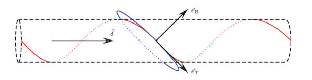
As an example of a vector function, we investigate $\mathbf{r}(t)$, the path of a point as a function of the time $t$. Thus we want to consider also the velocity $\mathbf{v}=\dot{\mathbf{r}}$ and the acceleration $\mathbf{a}=\ddot{\mathbf{r}}$ rather generally. The time is not important for the trajectories as geometrical lines. Therefore, instead of the time $t$ we introduce the path length $s$ as a parameter and exploit $\mathrm{d} s=|\mathrm{d} \mathbf{r}|=v \mathrm{~d} t$.
We now take three mutually perpendicular unit vectors $\mathbf{e}{\mathrm{T}}, \mathbf{e}{\mathrm{N}}$, and $\mathbf{e}{\mathrm{B}}$, which are attached to every point on the trajectory. Here $\mathbf{e}{\mathrm{T}}$ has the direction of $\mathbf{v}$ :
tangent vector $\quad \mathbf{e}{\mathrm{T}} \equiv \frac{\mathrm{d} \mathbf{r}}{\mathrm{d} s}=\frac{\mathbf{v}}{v}$ For a straight path, this vector is already sufficient for the description. But in general the path curvature $\quad \kappa \equiv\left|\frac{\mathrm{d} \mathbf{e}{\mathrm{T}}}{\mathrm{d} s}\right|=\left|\frac{\mathrm{d}^{2} \mathbf{r}}{\mathrm{d} s^{2}}\right|$
is different from zero. In order to get more insight into this parameter we consider a plane curve of constant curvature, namely, the circle with $s=R \varphi$. For $\mathbf{r}(\varphi)=\mathbf{r}{0}+$ $R\left(\cos \varphi \mathbf{e}{x}+\sin \varphi \mathbf{e}{y}\right)$, we have $\kappa=\left|\mathrm{d}^{2} \mathbf{r} / \mathrm{d}(R \varphi)^{2}\right|=R^{-1}$. Instead of the curvature $\kappa$, its reciprocal, the curvature radius $R \equiv \frac{1}{\kappa}$, can also be used to determine the curve. Hence as a further unit vector we have the normal vector $\quad \mathbf{e}{\mathrm{N}} \equiv R \frac{\mathbf{d} \mathbf{e}_{\mathrm{T}}}{\mathrm{d} s}=R \frac{\mathrm{d}^{2} \mathbf{r}}{\mathrm{d} s^{2}}$
理论力学代考
物理代写|理论力学代写theoretical mechanics代考|Space and Time
空间和时间是两个基本概念,在康德看来,它们先天地或先天地决定了所有经验的形式,从而使经验本身成为可 能: 只有在空间和时间中,我们才能安排我们的感觉。[根据进化认知的学说,我们与生倶来的东西是通过适应我 们的环境而在系统发育上发展起来的。这就是为什么我们只注意到这些”不言而喻”的概念在特殊情况下的不足之 处,例如,对于接近光速的速度 $\left(c_{0}\right)$ 或普朗克量子级的动作 $h$. 我们将在稍后的电磁学和量子力学中解决这些”奇怪” 的情况。目前,我们希望确保我们能够处理我们熟悉的环境。]
为此,我们引入了一个连续参数 $t$. 像所有其他物理量一样,它由数字和单位组成(例如,一秒 $1 \mathrm{~s}=1 \mathrm{~min} / 60$ $-1 \mathrm{~h} / 3600$ ) 。单位越大,数字越小。物理量不依赖于物理量之间的类似单位方程。然而,有时会看到相反的情 况,例如: “我们选择单位使得光速 $c$ 假定值为 1 “。事实上,速度的概念因此而改变,因此速度代替了速度 $v$ ,比例 $v / c$ 这里取为速度,并且 $c t$ 作为时间或 $x / c$ 作为长度。
零时 $(t=0)$ 可以任意选择,因为基本上只有时间差,即一个过程的持续时间,是重要的。时间上的差异化 $(\mathrm{d} / \mathrm{d} t)$ 通常在微分数量上用一个点标记,即 $\mathrm{d} x / \mathrm{d} t \equiv \dot{x}$.
在空旷的空间中,每个方向都是等价的。在这里,我们也可以自由选择零点,并从该点开始,通过位置向量以无坐 标表示法确定其他点的位置r,它固定了所考虑点的距离和方向。当我们想要利用假设的空间同质性时,这种无坐 标类型的符号特别有利。然而,通常会出现一些情况(即,当存在轴对称或球对称时),最好在特殊坐标中处理这 些情况。我们可以自由选择坐标系。我们只要求它唯一地确定所有位置。这一点我们将在下一节中讨论。
物理代写|理论力学代写theoretical mechanics代考|Vector Algebra
从两个向量 $\mathbf{a}$ 和 $\mathbf{b}$, 他们的总和 $\mathbf{a}+\mathbf{b}$ 可以根据平行四边形的构造 (作为对角线) 形成,如图 $1.1$ 所示。由此遵㑑向 量加法的交换结合律:
$$
\mathbf{a}+\mathbf{b}=\mathbf{b}+\mathbf{a}, \quad(\mathbf{a}+\mathbf{b})+\mathbf{c}=\mathbf{a}+(\mathbf{b}+\mathbf{c})
$$
向量 $\mathrm{a}$ 与标量 (即无方向) 因子的乘积 $\alpha$ 被理解为向量 $\alpha \mathbf{a}=\mathbf{a} \alpha$ 同样 (对于 $\alpha<0$ 相反) 方向和价值 $|\alpha| a$. 特别 是,一个和 $-\mathbf{a}$ 具有相同的值,但方向相反。为了 $\alpha=0$ 零向量 0 结果,长度为 0 ,方向末定。
标量积 (内积) $\mathbf{a} \cdot \mathbf{b}$ 两个向量的和b是它们的值乘以封闭角的余弦的乘积 $\phi_{a b}$ (见图 $1.2$ 左):
$$
\mathbf{a} \cdot \mathbf{b} \equiv a b \cos \phi_{a b}
$$
两个因子之间的点对于标量积很重要一一如果它缺失了,那么它就是两个向量的张量积,这将在 Sect. 1.2.4与 $\mathbf{a} \cdot \mathbf{b c} \neq \mathbf{a b} \cdot \mathbf{c}$ ,如果 $\mathbf{a}$ 和 $\mathbf{c}$ 有不同的方向,即,如果 $\mathbf{a}$ 不是的倍数 $\mathbf{c}$. 因此,一个有
$$
\mathbf{a} \cdot \mathbf{b}=\mathbf{b} \cdot \mathbf{a}
$$
和
$$
\mathbf{a} \cdot \mathbf{b}=0 \quad \Longleftrightarrow \quad \mathbf{a} \perp \mathbf{b} \text { or } a=0 \text { or } b=0
$$
如果两个向量相互垂直 $(\mathbf{a} \perp \mathbf{b})$ ,那么它们也被称为正交的。明显地, $\mathbf{a} \cdot \mathbf{a}=a^{2}$ 持有。值为 1 的向量称为单位 向量。在这里,它们用 e 表示。给定三个笛卡尔,即成对的垂直单位向量 $\mathbf{e} x, \mathbf{e} y, \mathbf{e} z$ ,所有向量都可以按照以下方 式分解:
$$
\mathbf{a}=\mathbf{e} x a_{x}+\mathbf{e} y a y+\mathbf{e} z a z
$$
使用笛卡尔分量
$$
a_{x} \equiv \mathbf{e} x \cdot \mathbf{a}, \quad a y \equiv \mathbf{e} y \cdot \mathbf{a}, \quad a z \equiv \mathbf{e}_{z} \cdot \mathbf{a} .
$$
物理代写|理论力学代写theoretical mechanics代考|Trajectories
如果一个向量依赖于一个参数,那么我们就说一个向量函数。向量函数 $\mathbf{a}(t)$ 是连续的 $t_{0}$ ,如果它倾向于 $\mathbf{a}\left(t_{0}\right)$ 为了 $t \rightarrow t_{0}$. 具有相同的限制 $t \rightarrow t_{0}$ ,向量微分 $\mathrm{da}$ 和一阶导数 $\mathrm{da} / \mathrm{d} t$ 介绍。这些量可以为每个笛卡尔分量形成,我们] 有
$$
\mathrm{d}(\mathbf{a}+\mathbf{b})=\mathrm{d} \mathbf{a}+\mathrm{d} \mathbf{b}, \quad \mathrm{d}(\alpha \mathbf{a})=\alpha \mathrm{d} \mathbf{a}+\mathbf{a d} \alpha \mathrm{d}(\mathbf{a} \cdot \mathbf{b})=\mathbf{a} \cdot \mathrm{d} \mathbf{b}+\mathbf{b} \cdot \mathrm{d} \mathbf{a}, \quad \mathrm{d}(\mathbf{a} \times \mathbf{b})=\mathbf{a} \times \mathrm{d} \mathbf{b}-\mathbf{b} \times \mathrm{d}
$$
明显地, $\mathbf{a} \cdot \mathrm{d} \mathbf{a} / \mathrm{d} t=\frac{1}{2} \mathrm{~d}(\mathbf{a} \cdot \mathbf{a}) / \mathrm{d} t=\frac{1}{2} \mathrm{~d} a^{2} / \mathrm{d} t=a \mathrm{~d} a / \mathrm{d} t$ 持有。特别是单位向量的导数总是垂直于原始 向量一一如果它不消失的话。
作为向量函数的一个例子,我们研究 $\mathbf{r}(t)$, 作为时间函数的点的路径t. 因此,我们还想考虑速度 $\mathbf{v}=\dot{\mathbf{r}}$ 和加速度 $\mathbf{a}=\ddot{\mathbf{r}}$ 相当普遍。对于作为几何线的轨迹来说,时间并不重要。因此,而不是时间 $t$ 我们引入路径长度 $s$ 作为参数并 利用 $\mathrm{d} s=|\mathrm{d} \mathbf{r}|=v \mathrm{~d} t$.
我们现在取三个相互垂直的单位向量eT $\mathrm{eN}$ ,和 $e B$ ,它们附加到轨迹上的每个点。这里eT有方向 $v:$ 切向量 $\quad \mathbf{e T} \equiv \frac{\mathrm{dr}}{\mathrm{d} s}=\frac{\mathrm{v}}{v}$ 对于直线路径,这个向量已经足够描述了。但总的来说路径曲率 $\quad \kappa \equiv\left|\frac{\mathrm{deT}}{\mathrm{d} s}\right|=\left|\frac{\mathrm{d}^{2} \mathrm{r}}{\mathrm{d} s^{2}}\right|$ 不同于零。为了更深入地了解这个参数,我们考虑一个恒定曲率的平面曲线,即圆 $s=R \varphi$. 为了 $\mathbf{r}(\varphi)=\mathbf{r} 0+$ $R(\cos \varphi \mathbf{e} x+\sin \varphi \mathbf{e} y)$ ,我们有 $\kappa=\left|\mathrm{d}^{2} \mathbf{r} / \mathrm{d}(R \varphi)^{2}\right|=R^{-1}$. 而不是曲率 $\kappa$ ,它的倒数,曲率半径 $R \equiv \frac{1}{\kappa}$ ,也 可用于确定曲线。因此,作为进一步的单位向量,我们有法线向量 $\mathrm{eN} \equiv R \frac{\mathrm{de} \mathrm{T}}{\mathrm{d} s}=R \frac{\mathrm{d}^{2} \mathrm{r}}{\mathrm{d} s^{2}}$

统计代写请认准statistics-lab™. statistics-lab™为您的留学生涯保驾护航。
金融工程代写
金融工程是使用数学技术来解决金融问题。金融工程使用计算机科学、统计学、经济学和应用数学领域的工具和知识来解决当前的金融问题,以及设计新的和创新的金融产品。
非参数统计代写
非参数统计指的是一种统计方法,其中不假设数据来自于由少数参数决定的规定模型;这种模型的例子包括正态分布模型和线性回归模型。
广义线性模型代考
广义线性模型(GLM)归属统计学领域,是一种应用灵活的线性回归模型。该模型允许因变量的偏差分布有除了正态分布之外的其它分布。
术语 广义线性模型(GLM)通常是指给定连续和/或分类预测因素的连续响应变量的常规线性回归模型。它包括多元线性回归,以及方差分析和方差分析(仅含固定效应)。
有限元方法代写
有限元方法(FEM)是一种流行的方法,用于数值解决工程和数学建模中出现的微分方程。典型的问题领域包括结构分析、传热、流体流动、质量运输和电磁势等传统领域。
有限元是一种通用的数值方法,用于解决两个或三个空间变量的偏微分方程(即一些边界值问题)。为了解决一个问题,有限元将一个大系统细分为更小、更简单的部分,称为有限元。这是通过在空间维度上的特定空间离散化来实现的,它是通过构建对象的网格来实现的:用于求解的数值域,它有有限数量的点。边界值问题的有限元方法表述最终导致一个代数方程组。该方法在域上对未知函数进行逼近。[1] 然后将模拟这些有限元的简单方程组合成一个更大的方程系统,以模拟整个问题。然后,有限元通过变化微积分使相关的误差函数最小化来逼近一个解决方案。
tatistics-lab作为专业的留学生服务机构,多年来已为美国、英国、加拿大、澳洲等留学热门地的学生提供专业的学术服务,包括但不限于Essay代写,Assignment代写,Dissertation代写,Report代写,小组作业代写,Proposal代写,Paper代写,Presentation代写,计算机作业代写,论文修改和润色,网课代做,exam代考等等。写作范围涵盖高中,本科,研究生等海外留学全阶段,辐射金融,经济学,会计学,审计学,管理学等全球99%专业科目。写作团队既有专业英语母语作者,也有海外名校硕博留学生,每位写作老师都拥有过硬的语言能力,专业的学科背景和学术写作经验。我们承诺100%原创,100%专业,100%准时,100%满意。
随机分析代写
随机微积分是数学的一个分支,对随机过程进行操作。它允许为随机过程的积分定义一个关于随机过程的一致的积分理论。这个领域是由日本数学家伊藤清在第二次世界大战期间创建并开始的。
时间序列分析代写
随机过程,是依赖于参数的一组随机变量的全体,参数通常是时间。 随机变量是随机现象的数量表现,其时间序列是一组按照时间发生先后顺序进行排列的数据点序列。通常一组时间序列的时间间隔为一恒定值(如1秒,5分钟,12小时,7天,1年),因此时间序列可以作为离散时间数据进行分析处理。研究时间序列数据的意义在于现实中,往往需要研究某个事物其随时间发展变化的规律。这就需要通过研究该事物过去发展的历史记录,以得到其自身发展的规律。
回归分析代写
多元回归分析渐进(Multiple Regression Analysis Asymptotics)属于计量经济学领域,主要是一种数学上的统计分析方法,可以分析复杂情况下各影响因素的数学关系,在自然科学、社会和经济学等多个领域内应用广泛。
MATLAB代写
MATLAB 是一种用于技术计算的高性能语言。它将计算、可视化和编程集成在一个易于使用的环境中,其中问题和解决方案以熟悉的数学符号表示。典型用途包括:数学和计算算法开发建模、仿真和原型制作数据分析、探索和可视化科学和工程图形应用程序开发,包括图形用户界面构建MATLAB 是一个交互式系统,其基本数据元素是一个不需要维度的数组。这使您可以解决许多技术计算问题,尤其是那些具有矩阵和向量公式的问题,而只需用 C 或 Fortran 等标量非交互式语言编写程序所需的时间的一小部分。MATLAB 名称代表矩阵实验室。MATLAB 最初的编写目的是提供对由 LINPACK 和 EISPACK 项目开发的矩阵软件的轻松访问,这两个项目共同代表了矩阵计算软件的最新技术。MATLAB 经过多年的发展,得到了许多用户的投入。在大学环境中,它是数学、工程和科学入门和高级课程的标准教学工具。在工业领域,MATLAB 是高效研究、开发和分析的首选工具。MATLAB 具有一系列称为工具箱的特定于应用程序的解决方案。对于大多数 MATLAB 用户来说非常重要,工具箱允许您学习和应用专业技术。工具箱是 MATLAB 函数(M 文件)的综合集合,可扩展 MATLAB 环境以解决特定类别的问题。可用工具箱的领域包括信号处理、控制系统、神经网络、模糊逻辑、小波、仿真等。