如果你也在 怎样代写量子场论Quantum field theory这个学科遇到相关的难题,请随时右上角联系我们的24/7代写客服。
在理论物理学中,量子场论(QFT)是一个理论框架,它结合了经典场论、狭义相对论和量子力学。QFT在粒子物理学中被用来构建亚原子粒子的物理模型,在凝聚态物理学中被用来构建类粒子的模型。
statistics-lab™ 为您的留学生涯保驾护航 在代写量子场论Quantum field theory方面已经树立了自己的口碑, 保证靠谱, 高质且原创的统计Statistics代写服务。我们的专家在代写量子场论Quantum field theory代写方面经验极为丰富,各种代写量子场论Quantum field theory相关的作业也就用不着说。
我们提供的量子场论Quantum field theory及其相关学科的代写,服务范围广, 其中包括但不限于:
- Statistical Inference 统计推断
- Statistical Computing 统计计算
- Advanced Probability Theory 高等概率论
- Advanced Mathematical Statistics 高等数理统计学
- (Generalized) Linear Models 广义线性模型
- Statistical Machine Learning 统计机器学习
- Longitudinal Data Analysis 纵向数据分析
- Foundations of Data Science 数据科学基础
物理代写|量子场论代写Quantum field theory代考|Path Integrals in Quantum and Statistical Mechanics
Already back in 1933 , Dirac asked himself whether the classical Lagrangian and action are as significant in quantum mechanics as they are in classical mechanics $[1,2]$. He observed that for simple systems, the probability amplitude
$$
K\left(t, q^{\prime}, q\right)=\left\langle q^{\prime}\left|\mathrm{e}^{-\mathrm{i} \hat{A} t / h}\right| q\right\rangle
$$
for the propagation from a point with coordinate $q$ to another point with coordinate $q^{\prime}$ in time $t$ is given by
$$
K\left(t, q^{\prime}, q\right) \propto \mathrm{e}^{\mathrm{i} S\left[q_{\mathrm{cl}}\right] / h}
$$
where $q_{\mathrm{cl}}$ denotes the classical trajectory from $q$ to $q^{\prime}$. In the exponent the action of this trajectory enters as a multiple of Planck’s reduced constant $h$. For a free particle with Lagrangian
$$
L_{0}=\frac{m}{2} \dot{q}^{2}
$$ the formula $(2.2)$ is verified easily: A free particle moves with constant velocity $\left(q^{\prime}-q\right) / t$ from $q$ to $q^{\prime}$ and the action of the classical trajectory is
$$
S\left[q_{\mathrm{cl}}\right]=\int_{0}^{t} \mathrm{~d} s L_{0}\left[q_{\mathrm{cl}}(s)\right]=\frac{m}{2 t}\left(q^{\prime}-q\right)^{2}
$$
The factor of proportionality in $(2.2)$ is then uniquely fixed by the condition $\mathrm{e}^{-\mathrm{i} \hat{H} t / \hbar} \longrightarrow 1$ for $t \rightarrow 0$ which in position space reads
$$
\lim {t \rightarrow 0} K\left(t, q^{\prime}, q\right)=\delta\left(q^{\prime}, q\right) $$ Alternatively, it is fixed by the property $\mathrm{e}^{-\mathrm{i} \hat{H} t / h} \mathrm{e}^{-\mathrm{i} \hat{H} s / h}=\mathrm{e}^{-\mathrm{i} \hat{H}(t+s) / h}$ that takes the form $$ \int \mathrm{d} u K\left(t, q^{\prime}, u\right) K(s, u, q)=K\left(t+s, q^{\prime}, q\right) $$ in position space. Thus, the correct free particle propagator on a line is given by $$ K{0}\left(t, q^{\prime} \cdot q\right)=\left(\frac{m}{2 \pi \mathrm{i} \hbar t}\right)^{1 / 2} \mathrm{c}^{\mathrm{i} m\left(q^{\prime}-q\right)^{2} / 2 h t}
$$
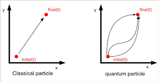
Similar results hold for the harmonic oscillator or systems for which $\langle\hat{q}(t)\rangle$ fulfills the classical equation of motion. For such systems $\left\langle V^{\prime}(\hat{q})\right\rangle=V^{\prime}(\langle\hat{q}\rangle)$ holds true. However, for general systems, the simple formula (2.2) must be extended, and it was Feynman who discovered this extension back in 1948. He realized that all paths from $q$ to $q^{\prime}$ (and not only the classical path) contribute to the propagator. This means that in quantum mechanics a particle can potentially move on any path $q(s)$ from the initial to the final destination,
$$
q(0)=q \quad \text { and } \quad q(t)=q^{\prime}
$$
物理代写|量子场论代写Quantum field theory代考|Recalling Quantum Mechanics
There are two well-established ways to quantize a classical system: canonical quantization and path integral quantization. For completeness and later use, we recall the main steps of canonical quantization both in Schrödinger’s wave mechanics and Heisenberg’s matrix mechanics.
A classical system is described by its coordinates $\left{q^{i}\right}$ and momenta $\left{p_{i}\right}$ on phase space $\Gamma$. An observable $O$ is a real-valued function on $\Gamma$. Examples are the coordinates on phase space and the energy $H(q, p)$. We assume that phase space comes along with a symplectic structure and has local coordinates with Poisson brackets
$$
\left{q^{i}, p_{j}\right}=\delta_{j}^{i}
$$
The brackets are extended to observables on through antisymmetry and the derivation rule ${O P, Q}=O{P, Q}+{O, Q} P$. The evolution in time of an observable is determined by
$$
\dot{O}={O, H}, \quad \text { e.g. } \quad \dot{q}^{i}=\left{q^{i}, H\right} \quad \text { and } \quad \dot{p}{i}=\left{p{i}, H\right}
$$
In the canonical quantization, functions on phase space are mapped to operators, and the Poisson brackets of two functions become commutators of the associated operators:
$$
O(q, p) \rightarrow \hat{O}(\hat{q}, \hat{p}) \quad \text { and } \quad{O, P} \longrightarrow \frac{1}{\mathrm{i} \hbar}[\hat{O}, \hat{P}]
$$
The time evolution of an (not explicitly time-dependent) observable is determined by Heisenberg’s equation
$$
\frac{\mathrm{d} \hat{O}}{\mathrm{~d} t}=\frac{\mathrm{i}}{\hbar}[\hat{H}, \hat{O}]
$$
In particular the phase space coordinates $\left(q^{l}, p_{i}\right)$ become operators with commutation relations $\left[\hat{q}^{i}, \hat{p}{j}\right]=\mathrm{i} \hbar \delta{j}^{i}$, and their time evolution is determined by
$$
\frac{\mathrm{d} \hat{q}^{i}}{\mathrm{~d} t}=\frac{\mathrm{i}}{\hbar}\left[\hat{H}, \hat{q}^{i}\right] \quad \text { and } \quad \frac{\mathrm{d} \hat{p}{i}}{\mathrm{~d} t}=\frac{\mathrm{i}}{\hbar}\left[\hat{H}, \hat{p}{i}\right]
$$
For a system of non-relativistic and spinless particles, the Hamiltonian reads
$$
\hat{H}=\hat{H}{0}+\hat{V} \quad \text { with } \quad \hat{H}{0}=\frac{1}{2 m} \sum \hat{p}{i}^{2} $$ and one arrives at Heisenberg’s equations of motion $$ \frac{\mathrm{d} \hat{q}^{i}}{\mathrm{~d} t}=\frac{\hat{p}{i}}{m} \quad \text { and } \quad \frac{\mathrm{d} \hat{p}{i}}{\mathrm{~d} t}=-\hat{V}{, i}
$$
Observables are represented by Hermitian operators on a Hilbert space $\mathscr{H}$, whose elements characterize the states of the system:
$$
\hat{O}(\hat{q}, \hat{p}): \mathcal{H} \longrightarrow \mathcal{H}
$$
Consider a particle confined to an endless wire. Its Hilbert space is $\mathcal{H}=L_{2}(\mathbb{R})$, and its position and momentum operator are represented in position space as
$$
(\hat{q} \psi)(q)=q \psi(q) \quad \text { and } \quad(\hat{p} \psi)(q)=\frac{\hbar}{i} \partial_{q} \psi(q)
$$
物理代写|量子场论代写Quantum field theory代考|Feynman–Kac Formula
We shall derive Feynman’s path integral representation for the unitary time evolution operator $\exp (-\mathrm{i} \hat{H} t)$ as well as Kac’s path integral representation for the positive operator $\exp (-\hat{H} \tau)$. Thereby we shall utilize the product formula of Trotter. In case of matrices, this formula was already verified by Lie and has the form:
Theorem 2.1 (Lie’s Theorem) For two matrices $\mathrm{A}$ and $\mathrm{B}$
$$
\mathrm{e}^{\mathrm{A}+\mathrm{B}}=\lim {n \rightarrow \infty}\left(\mathrm{e}^{\mathrm{A} / n} \mathrm{e}^{\mathrm{B} / n}\right)^{n} $$ To prove this theorem, we define for each $n$ the two matrices $\mathrm{S}{n}:=\exp (\mathrm{A} / n+\mathrm{B} / n)$ and $\mathrm{T}{n}:=\exp (\mathrm{A} / n) \exp (\mathrm{B} / n)$ and telescope the difference of their $n$ ‘th powers, $$ \mathrm{S}{n}^{n}-\mathrm{T}{n}^{n}=\mathrm{S}{n}^{n-1}\left(\mathrm{~S}{n}-\mathrm{T}{n}\right)+\mathrm{S}{n}^{n-2}\left(\mathrm{~S}{n}-\mathrm{T}{n}\right) \mathrm{T}{n}+\cdots+\left(\mathrm{S}{n}-\mathrm{T}{n}\right) \mathrm{T}{n}^{n-1} $$ Now we choose any (sub-multiplicative) matrix norm, for example, the Frobenius norm. The triangle inequality together with $|X Y| \leq|X \mid| Y |$ imply the inequality $|\exp (X)| \leq \exp (|X|)$ such that $$ \left|\mathrm{S}{n}\right|,\left|\mathrm{T}{n}\right| \leq a^{1 / n} \quad \text { with } \quad a=\mathrm{e}^{|\mathrm{A}|+|\mathrm{B}|} $$ Thus we conclude $$ \left|\mathrm{S}{n}^{n}-\mathrm{T}{n}^{n}\right| \equiv\left|\mathrm{e}^{\mathrm{A}+B}-\left(\mathrm{e}^{\mathrm{A} / n} \mathrm{e}^{B / n}\right)^{n}\right| \leq n \times a^{(n-1) / n}\left|\mathrm{~S}{n}-\mathrm{T}{n}\right| $$ Finally, using $\mathrm{S}{n}-\mathrm{T}_{n}=-[\mathrm{A}, \mathrm{B}] / 2 n^{2}+O\left(1 / n^{3}\right)$, the product formula is verified for matrices. But the theorem also holds for self-adjoint operators.
Theorem $2.2$ (Trotter’s Theorem) If $\hat{A}$ and $\hat{B}$ are self-adjoint operators and $\hat{A}+$ $\hat{B}$ is essentially self-adjoint on the intersection $\mathscr{D}$ of their domains, then
$$
\mathrm{e}^{-\mathrm{i} t(\hat{A}+\hat{B})}=s-\lim {n \rightarrow \infty}\left(\mathrm{e}^{-\mathrm{i} t \hat{A} / n} \mathrm{e}^{-\mathrm{i} t \hat{B} / n}\right)^{n} $$ If in addition $\hat{A}$ and $\hat{B}$ are bounded from below, then $$ \mathrm{e}^{-\tau(\hat{A}+\hat{B})}=s-\lim {n \rightarrow \infty}\left(\mathrm{e}^{-\tau \hat{A} / n} \mathrm{e}^{-\tau \hat{B} / n}\right)^{n}
$$
The operators need not be bounded and the convergence is with respect to the strong operator topology. For operators $\hat{A}{n}$ and $\hat{A}$ on a common domain $\mathscr{D}$ in the Hilbert space, we have s- $\lim {n \rightarrow \infty} \hat{A}{n}=\hat{A}$ iff $\left|\hat{A}{n} \psi-\hat{A} \psi\right| \rightarrow 0$ for all $\psi \in \mathscr{D}$. Formula (2.27) is used in quantum mechanics, and formula $(2.28)$ finds its application in statistical physics and the Euclidean formulation of quantum mechanics [16].
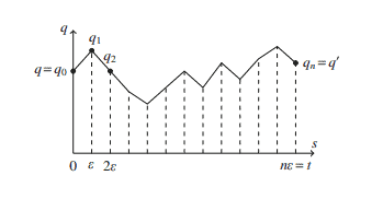
Let us assume that $\hat{H}$ can be written as $\hat{H}=\hat{H}{0}+\hat{V}$ and apply the product formula to the evolution kernel in (2.22). With $\varepsilon=t / n$ and $\hbar=1$, we obtain $$ \begin{aligned} K\left(t, q^{\prime}, q\right) &=\lim {n \rightarrow \infty}\left\langle q^{\prime}\left|\left(\mathrm{e}^{-\mathrm{i} \varepsilon \hat{H}{0}} \mathrm{e}^{-\mathrm{i} \varepsilon \hat{V}}\right)^{n}\right| q\right\rangle \ &=\lim {n \rightarrow \infty} \int \mathrm{d} q_{1} \cdots \mathrm{d} q_{n-1} \prod_{j=0}^{j=n-1}\left|q_{j+1}\right| \mathrm{e}^{-\mathrm{i} \varepsilon \hat{H}{0}} \mathrm{e}^{-i \varepsilon \hat{V}}\left|q{j}\right\rangle
\end{aligned}
$$
where we repeatedly inserted the resolution of the identity $(2.21)$ and denoted the initial and final point by $q_{0}=q$ and $q_{n}=q^{\prime}$, respectively. The potential $\hat{V}$ is diagonal in position space such that
$$
\left\langle q_{j+1}\left|\mathrm{e}^{-\mathrm{i} \varepsilon \hat{H}{0}} \mathrm{e}^{-\mathrm{i} \varepsilon \hat{V}}\right| q{j}\right\rangle=\left\langle q_{j+1}\left|\mathrm{e}^{-\mathrm{i} \varepsilon \hat{H}{0}}\right| q{j}\right\rangle \mathrm{e}^{-\mathrm{i} \varepsilon V\left(q_{j}\right)}
$$
量子场论代考
物理代写|量子场论代写Quantum field theory代考|Path Integrals in Quantum and Statistical Mechanics
早在 1933 年,狄拉克就问自己,经典拉格朗日算子和作用在量子力学中是否与在经典力学中一样重要[1,2]. 他观察到,对于简单系统,概率幅
ķ(吨,q′,q)=⟨q′|和−一世一个^吨/H|q⟩
对于从具有坐标的点的传播q到另一个坐标点q′及时吨是(谁)给的
ķ(吨,q′,q)∝和一世小号[qCl]/H
在哪里qCl表示来自的经典轨迹q至q′. 在指数中,该轨迹的作用作为普朗克约化常数的倍数进入H. 对于具有拉格朗日的自由粒子
大号0=米2q˙2公式(2.2)容易验证:自由粒子以恒定速度运动(q′−q)/吨从q至q′经典轨迹的作用是
小号[qCl]=∫0吨 ds大号0[qCl(s)]=米2吨(q′−q)2
比例系数(2.2)然后由条件唯一固定和−一世H^吨/ℏ⟶1为了吨→0在位置空间中读取
林吨→0ķ(吨,q′,q)=d(q′,q)或者,它由属性固定和−一世H^吨/H和−一世H^s/H=和−一世H^(吨+s)/H采取形式
∫d在ķ(吨,q′,在)ķ(s,在,q)=ķ(吨+s,q′,q)在位置空间。因此,一条线上正确的自由粒子传播子由下式给出
ķ0(吨,q′⋅q)=(米2圆周率一世ℏ吨)1/2C一世米(q′−q)2/2H吨
类似的结果适用于谐波振荡器或系统⟨q^(吨)⟩满足经典的运动方程。对于这样的系统⟨在′(q^)⟩=在′(⟨q^⟩)成立。然而,对于一般系统,必须扩展简单的公式(2.2),而费曼早在 1948 年就发现了这个扩展。他意识到所有从q至q′(不仅是经典路径)有助于传播者。这意味着在量子力学中,粒子可以在任何路径上移动q(s)从最初的目的地到最终的目的地,
q(0)=q 和 q(吨)=q′
物理代写|量子场论代写Quantum field theory代考|Recalling Quantum Mechanics
量化经典系统有两种行之有效的方法:规范量化和路径积分量化。为了完整性和以后的使用,我们回顾一下薛定谔的波力学和海森堡的矩阵力学中规范量化的主要步骤。
经典系统由其坐标描述\left{q^{i}\right}\left{q^{i}\right}和动量\left{p_{i}\right}\left{p_{i}\right}在相空间Γ. 一个可观察的○是一个实值函数Γ. 例子是相空间上的坐标和能量H(q,p). 我们假设相空间带有一个辛结构并且具有泊松括号的局部坐标
\left{q^{i}, p_{j}\right}=\delta_{j}^{i}\left{q^{i}, p_{j}\right}=\delta_{j}^{i}
括号通过反对称和推导规则扩展到可观察量○磷,问=○磷,问+○,问磷. 可观测量的时间演化由下式决定
\dot{O}={O, H}, \quad \text { 例如} \quad \dot{q}^{i}=\left{q^{i}, H\right} \quad \text { 和} \quad \dot{p}{i}=\left{p{i}, H\right}\dot{O}={O, H}, \quad \text { 例如} \quad \dot{q}^{i}=\left{q^{i}, H\right} \quad \text { 和} \quad \dot{p}{i}=\left{p{i}, H\right}
在规范量化中,相空间上的函数被映射到算子,两个函数的泊松括号成为相关算子的交换子:
○(q,p)→○^(q^,p^) 和 ○,磷⟶1一世ℏ[○^,磷^]
(不是明确的时间相关的)可观测的时间演化由海森堡方程确定
d○^ d吨=一世ℏ[H^,○^]
特别是相空间坐标(ql,p一世)成为有交换关系的算子[q^一世,p^j]=一世ℏdj一世, 它们的时间演化由下式决定
dq^一世 d吨=一世ℏ[H^,q^一世] 和 dp^一世 d吨=一世ℏ[H^,p^一世]
对于非相对论和无自旋粒子系统,哈密顿量为
H^=H^0+在^ 和 H^0=12米∑p^一世2一个到达海森堡的运动方程
dq^一世 d吨=p^一世米 和 dp^一世 d吨=−在^,一世
Observables 由希尔伯特空间上的 Hermitian 算子表示H,其元素表征系统的状态:
○^(q^,p^):H⟶H
考虑一个被限制在无限线中的粒子。它的希尔伯特空间是H=大号2(R),其位置和动量算子在位置空间中表示为
(q^ψ)(q)=qψ(q) 和 (p^ψ)(q)=ℏ一世∂qψ(q)
物理代写|量子场论代写Quantum field theory代考|Feynman–Kac Formula
我们将推导出酉时间演化算子的费曼路径积分表示经验(−一世H^吨)以及正算子的 Kac 路径积分表示经验(−H^τ). 因此我们将利用Trotter的产品配方。在矩阵的情况下,这个公式已经被 Lie 验证并具有形式:
Theorem 2.1 (Lie’s Theorem) 对于两个矩阵一个和乙
和一个+乙=林n→∞(和一个/n和乙/n)n为了证明这个定理,我们定义每个n两个矩阵小号n:=经验(一个/n+乙/n)和吨n:=经验(一个/n)经验(乙/n)并望远镜他们的差异n的权力,
小号nn−吨nn=小号nn−1( 小号n−吨n)+小号nn−2( 小号n−吨n)吨n+⋯+(小号n−吨n)吨nn−1现在我们选择任何(子乘法)矩阵范数,例如 Frobenius 范数。三角不等式与|X是|≤|X∣|是|暗示不等式|经验(X)|≤经验(|X|)这样
|小号n|,|吨n|≤一个1/n 和 一个=和|一个|+|乙|因此我们得出结论
|小号nn−吨nn|≡|和一个+乙−(和一个/n和乙/n)n|≤n×一个(n−1)/n| 小号n−吨n|最后,使用小号n−吨n=−[一个,乙]/2n2+○(1/n3),乘积公式针对矩阵进行验证。但该定理也适用于自伴算子。
定理2.2(特罗特定理)如果一个^和乙^是自伴算子和一个^+ 乙^在交点上本质上是自伴的D他们的域,然后
和−一世吨(一个^+乙^)=s−林n→∞(和−一世吨一个^/n和−一世吨乙^/n)n如果另外一个^和乙^是从下方有界的,那么
和−τ(一个^+乙^)=s−林n→∞(和−τ一个^/n和−τ乙^/n)n
算子不需要有界,收敛与强算子拓扑有关。对于运营商一个^n和一个^在一个共同的领域D在希尔伯特空间中,我们有 s-林n→∞一个^n=一个^当且当|一个^nψ−一个^ψ|→0对所有人ψ∈D. 公式(2.27)用于量子力学,公式(2.28)发现其在统计物理学和量子力学的欧几里得公式中的应用[16]。
让我们假设H^可以写成H^=H^0+在^并将乘积公式应用于(2.22)中的进化核。和e=吨/n和ℏ=1, 我们获得
ķ(吨,q′,q)=林n→∞⟨q′|(和−一世eH^0和−一世e在^)n|q⟩ =林n→∞∫dq1⋯dqn−1∏j=0j=n−1|qj+1|和−一世eH^0和−一世e在^|qj⟩
我们反复插入身份的解析(2.21)并用q0=q和qn=q′, 分别。潜力在^在位置空间中是对角线使得
⟨qj+1|和−一世eH^0和−一世e在^|qj⟩=⟨qj+1|和−一世eH^0|qj⟩和−一世e在(qj)

统计代写请认准statistics-lab™. statistics-lab™为您的留学生涯保驾护航。
金融工程代写
金融工程是使用数学技术来解决金融问题。金融工程使用计算机科学、统计学、经济学和应用数学领域的工具和知识来解决当前的金融问题,以及设计新的和创新的金融产品。
非参数统计代写
非参数统计指的是一种统计方法,其中不假设数据来自于由少数参数决定的规定模型;这种模型的例子包括正态分布模型和线性回归模型。
广义线性模型代考
广义线性模型(GLM)归属统计学领域,是一种应用灵活的线性回归模型。该模型允许因变量的偏差分布有除了正态分布之外的其它分布。
术语 广义线性模型(GLM)通常是指给定连续和/或分类预测因素的连续响应变量的常规线性回归模型。它包括多元线性回归,以及方差分析和方差分析(仅含固定效应)。
有限元方法代写
有限元方法(FEM)是一种流行的方法,用于数值解决工程和数学建模中出现的微分方程。典型的问题领域包括结构分析、传热、流体流动、质量运输和电磁势等传统领域。
有限元是一种通用的数值方法,用于解决两个或三个空间变量的偏微分方程(即一些边界值问题)。为了解决一个问题,有限元将一个大系统细分为更小、更简单的部分,称为有限元。这是通过在空间维度上的特定空间离散化来实现的,它是通过构建对象的网格来实现的:用于求解的数值域,它有有限数量的点。边界值问题的有限元方法表述最终导致一个代数方程组。该方法在域上对未知函数进行逼近。[1] 然后将模拟这些有限元的简单方程组合成一个更大的方程系统,以模拟整个问题。然后,有限元通过变化微积分使相关的误差函数最小化来逼近一个解决方案。
tatistics-lab作为专业的留学生服务机构,多年来已为美国、英国、加拿大、澳洲等留学热门地的学生提供专业的学术服务,包括但不限于Essay代写,Assignment代写,Dissertation代写,Report代写,小组作业代写,Proposal代写,Paper代写,Presentation代写,计算机作业代写,论文修改和润色,网课代做,exam代考等等。写作范围涵盖高中,本科,研究生等海外留学全阶段,辐射金融,经济学,会计学,审计学,管理学等全球99%专业科目。写作团队既有专业英语母语作者,也有海外名校硕博留学生,每位写作老师都拥有过硬的语言能力,专业的学科背景和学术写作经验。我们承诺100%原创,100%专业,100%准时,100%满意。
随机分析代写
随机微积分是数学的一个分支,对随机过程进行操作。它允许为随机过程的积分定义一个关于随机过程的一致的积分理论。这个领域是由日本数学家伊藤清在第二次世界大战期间创建并开始的。
时间序列分析代写
随机过程,是依赖于参数的一组随机变量的全体,参数通常是时间。 随机变量是随机现象的数量表现,其时间序列是一组按照时间发生先后顺序进行排列的数据点序列。通常一组时间序列的时间间隔为一恒定值(如1秒,5分钟,12小时,7天,1年),因此时间序列可以作为离散时间数据进行分析处理。研究时间序列数据的意义在于现实中,往往需要研究某个事物其随时间发展变化的规律。这就需要通过研究该事物过去发展的历史记录,以得到其自身发展的规律。
回归分析代写
多元回归分析渐进(Multiple Regression Analysis Asymptotics)属于计量经济学领域,主要是一种数学上的统计分析方法,可以分析复杂情况下各影响因素的数学关系,在自然科学、社会和经济学等多个领域内应用广泛。
MATLAB代写
MATLAB 是一种用于技术计算的高性能语言。它将计算、可视化和编程集成在一个易于使用的环境中,其中问题和解决方案以熟悉的数学符号表示。典型用途包括:数学和计算算法开发建模、仿真和原型制作数据分析、探索和可视化科学和工程图形应用程序开发,包括图形用户界面构建MATLAB 是一个交互式系统,其基本数据元素是一个不需要维度的数组。这使您可以解决许多技术计算问题,尤其是那些具有矩阵和向量公式的问题,而只需用 C 或 Fortran 等标量非交互式语言编写程序所需的时间的一小部分。MATLAB 名称代表矩阵实验室。MATLAB 最初的编写目的是提供对由 LINPACK 和 EISPACK 项目开发的矩阵软件的轻松访问,这两个项目共同代表了矩阵计算软件的最新技术。MATLAB 经过多年的发展,得到了许多用户的投入。在大学环境中,它是数学、工程和科学入门和高级课程的标准教学工具。在工业领域,MATLAB 是高效研究、开发和分析的首选工具。MATLAB 具有一系列称为工具箱的特定于应用程序的解决方案。对于大多数 MATLAB 用户来说非常重要,工具箱允许您学习和应用专业技术。工具箱是 MATLAB 函数(M 文件)的综合集合,可扩展 MATLAB 环境以解决特定类别的问题。可用工具箱的领域包括信号处理、控制系统、神经网络、模糊逻辑、小波、仿真等。