如果你也在 怎样代写产业经济学Industrial Economics这个学科遇到相关的难题,请随时右上角联系我们的24/7代写客服。
产业经济学是关于公司、行业和市场的研究。它研究各种规模的公司–从当地的角落商店到沃尔玛或乐购这样的跨国巨头。它还考虑了一系列的行业,如发电、汽车生产和餐馆。
statistics-lab™ 为您的留学生涯保驾护航 在代写产业经济学Industrial Economics方面已经树立了自己的口碑, 保证靠谱, 高质且原创的统计Statistics代写服务。我们的专家在代写产业经济学Industrial Economics代写方面经验极为丰富,各种代写产业经济学Industrial Economics相关的作业也就用不着说。
我们提供的产业经济学Industrial Economics及其相关学科的代写,服务范围广, 其中包括但不限于:
- Statistical Inference 统计推断
- Statistical Computing 统计计算
- Advanced Probability Theory 高等概率论
- Advanced Mathematical Statistics 高等数理统计学
- (Generalized) Linear Models 广义线性模型
- Statistical Machine Learning 统计机器学习
- Longitudinal Data Analysis 纵向数据分析
- Foundations of Data Science 数据科学基础
经济代写|产业经济学代写Industrial Economics代考|Debt risks accumulated to pin down industrial operation
Local debt risk remains high. During economic deceleration, the fiscal revenue growth will slow down and the expenditure will rise moderately under the influence of economic fundamentals, enlarging the scale of deficit and debt. Furthermore, the fact that local governments may execute debt financing on various financing platforms to maintain goals of local economic and social development and to accelerate infrastructure construction will initiate a new mode to stimulate economic growth by governments’ leveraging investment. When the government no long provides any guarantee for these debts, some of the debts will be transferred by financing platforms to debts payable by the government; as a result, the debts payable by the local government will increase. According to the results of national debt audit at the end of 2015, RMB $1.9$ trillion debts payable by the government fell due in 2015 . Excessive debt ratio of the local government will put local government under heavy pressure to discharge debts and will also easily lead to crisis of local government debts; in addition, due to different rates of local economic growth and different debt burden of provinces, it is likely to incur local debt crisis. Excessive local government debts may also lead to risk of local government’s bankruptcy and place strict restrictions on local government’s further financing and on continuous investment in infrastructure construction and thus compromise the growth of industrial economics.
Potential risk in industrial sectors remains high. In May 2016, the debt-to-asset ratio of industrial enterprises above designated size was $56.8 \%, 0.6$ percentage point higher than December 2015 , and the leverage ratio reached up to $131 \%$, which increased the operating risk of industrial sectors. It is noted that the excessively high leverage ratio of Chinese enterprises was questioned as the leverage ratio of foreign enterprises maintained at around $70 \%$. In effect, the leverage ratio of Chinese enterprises has been extremely high for many years, for it was closely related to Chinese economic reality: (i) high saving rate that means relatively adequate supply of capitals in China, and (ii) high leverage that results from two realistic bases – relatively lagging development of China’s capital market and credit financing used as the main financing channel by China’s industrial sectors. However, these two bases are slowly collapsing as the consumer savings declines and the capital market expands and plays more financing functions. In recent years, the de-leverage ratio of industrial enterprises has paced up, reducing from $178 \%$ at the beginning of 1998 to $128 \%$ at the end of December 2015 . The current uptrend of leverage has no realistic base. Furthermore, the local government’s debt risks are constantly discharged. China as a whole suffers a very high debt ratio, so the increasing leverage will intensify the risk pressure.
经济代写|产业经济学代写Industrial Economics代考|Prediction of Industrial Growth Trend
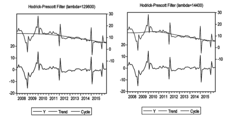
HP filtering method adopted in this report separates the growth trend of industrial value added year on year from cyclical factors to analyze roles of different factors in industrial value added. According to the results, the growth rate of industrial economics has slowed down since the year of 2010 ; the slowing growth rate has continued in the first half of 2016 but the decreasing amplitude was narrowing; and it is predicted that the industrial growth will highly likely hit the bottom in the second half of 2016
(1) Data source and interpolation of missing values
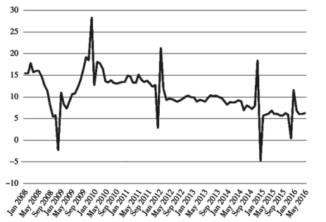
In this report, the value added year-on-year growth data of industries above designated size are used as observing indicators of industrial growth, with the samples ranging between January 2008 and June 2016 . Data are sourced from National Bureau of Statistics website. The industrial value added year-on-year growth rate is: (i) calculated by comparable prices, independent of price factors and free from price adjustment, and (ii) value added growth data of industries above designated size with January growth data missed, which needs interpolation. The traceability method is adopted in this report to interpolate data. Specific steps are as follows.
Firstly, the monthly year-on-year growth rate data and the monthly accumulative growth rate data of industrial value added as well as the monthly actual data in 2005 of industrial value added ${ }^{2}$ are obtained from National Bureau of Statistics website. Secondly, the monthly industrial value actually added in 2005 is used to figure out the monthly accumulative growth rates of industrial value added in 2005 . Thirdly, the monthly accumulative industrial value added in 2005 and the monthly accumulative growth rates of industrial value added in 2006 are used to calculate the monthly accumulative industrial value added in 2006 , and by analogy get the monthly accumulative industrial value added from 2007 to 2016 with January data missed. Fourthly, the monthly industrial value actually added in 2005 and the monthly year-on-year growth rates of industrial value added in 2006 are used to figure out the monthly industrial value actually added in 2006 , and by analogy get the monthly industrial value actually added from 2007 to 2016 with January data missed. Fifthly, the industrial values actually added in January from 2006 to 2013 are obtained by the accumulative number in February of industrial value added from 2006 to 2016 with January data missed minus the actual industrial value added in February from 2006 to 2016 . Finally, all monthly data calculated above are used to directly get the missing January data about the monthly year-on-year growth rates of industrial value added (Fig. 2.5).
经济代写|产业经济学代写Industrial Economics代考|Trend components
In order to separate the long-term trend factors from the cyclical (irregular) factors of industrial growth and obtain estimation of unobservable potential factors, either the moving average method or the frequency domain estimation method may be used for the original data of single time sequence; the filtering method has a unique advantage, i.e. simple, intuitive and easy for implementation, and can also avoid the problem caused by production function method, i.e. whether the product function can be stable in the economic transition period, and the problem caused by variable structure decomposition method, i.e. whether there exists the Phillips curve of conventional form in China. Therefore, the HP filtering method is adopted in this section to predict the growth trend of industrial economics.
The HP filtering de-trending method may regard economic operation as a certain combination of potential growth and short-term fluctuations and use metrological technology to decompose the actually output sequence into trend components and cyclical components; the former means potential output while the latter means output gap or fluctuation. For growth rate of industrial operation, the time sequence $y_{t}$ consists of industrial operation trend $g_{t}$ and industrial operation fluctuation $c_{t}$, namely:
$$
y_{t}=g_{t}+c_{t} \quad t=1, \ldots T
$$
Hodrick and Prescott $(1980,1997)^{3}$ designed HP filter by following the logarithm data moving average method. The filter can obtain a smooth sequence $g_{t}$ from the time sequence $y_{t}$, i.e. trend component, and $g_{t}$ is the solution to the formula below:
$$
\operatorname{Min}\left{\sum_{t=1}^{T}\left(y_{t}-g_{t}\right)^{2}+\lambda \sum_{t=1}^{T}\left[\left(g_{t}-g_{t-1}\right)\left(g_{t}-g_{t-2}\right)\right]\right}
$$
where, $\sum_{t=1}^{T}\left(y_{t}-g_{t}\right)^{2}$ represents fluctuations, $\sum_{t=1}^{T}\left[\left(g_{t}-g_{t-1}\right)\left(g_{t}-g_{t-2}\right)\right]$ represents trend, and $\lambda$ is smooth parameter with a positive value used to adjust proportions of fluctuation and trend. Selection of the smooth parameter $\lambda$ is an important problem in the HP filtering method. Different smooth parameters mean different filters that determine different fluctuating modes and smoothness. According to Hodrick and Prescott $(1980,1997)$, the value of smooth parameter is taken as 100 in processing annual data, as 1600 in processing quarterly data and as 14,400 in processing monthly data. According to Ravn and Uhlig (2002), ${ }^{4}$ the smooth parameter should be 4th power of the observed data frequency, i.e. $6.25$ for annual data, 1600 for quarterly data and 129,600 for monthly data. In this report, the data used are growth rates of industrial value added from January 2010 to September 2015, sourced from National Bureau of Statistics website. It is important to note that the missing data on growth rates of industrial value added in January on National Bureau of Statistics website are supplemented by point linear interpolation in this report. Above two types of filters are selected for use in this report: $\lambda=14,400$ and $\lambda=129,600$.
产业经济学代考
经济代写|产业经济学代写Industrial Economics代考|Debt risks accumulated to pin down industrial operation
地方债务风险仍然很高。经济减速期间,受经济基本面影响,财政收入增速放缓,支出适度增加,赤字和债务规模扩大。此外,地方政府为了维护地方经济社会发展目标,加快基础设施建设,可以通过各种融资平台进行债务融资,这将开启政府杠杆投资拉动经济增长的新模式。当政府不再为这些债务提供任何担保时,部分债务将通过融资平台转移为政府应付的债务;这样一来,地方政府应付的债务就会增加。根据 2015 年末国债审计结果,人民币1.92015年政府应付的万亿债务到期。地方政府负债率过高,将给地方政府带来沉重的债务清偿压力,也容易引发地方政府债务危机;此外,由于地方经济增速不同,各省债务负担不同,很可能引发地方债务危机。过多的地方政府债务还可能导致地方政府破产风险,对地方政府进一步融资和基础设施建设持续投资造成严格限制,从而影响产业经济增长。
工业领域的潜在风险仍然很高。2016年5月,规模以上工业企业资产负债率为56.8%,0.6比 2015 年 12 月 高 1 个 百分点 , 杠杆 率 达到131%,增加了工业板块的经营风险。值得注意的是,中国企业的杠杆率过高被质疑为外国企业的杠杆率维持在70%. 实际上,中国企业的杠杆率多年来一直处于极高水平,因为它与中国经济现实密切相关:(i)高储蓄率意味着中国的资本供应相对充足,(ii)高杠杆率意味着这源于两个现实基础——中国资本市场发展相对滞后和中国工业部门以信贷融资为主要融资渠道。然而,随着消费者储蓄下降和资本市场扩大并发挥更多融资功能,这两个基础正在慢慢崩溃。近年来,工业企业去杠杆率有所上升,从178%1998 年初至128%2015 年 12 月末。目前的杠杆上升趋势没有现实基础。此外,地方政府的债务风险也在不断释放。中国整体负债率非常高,杠杆率上升将加剧风险压力。
经济代写|产业经济学代写Industrial Economics代考|Prediction of Industrial Growth Trend
本报告采用HP过滤法,将工业增加值同比增长趋势与周期性因素分开,分析不同因素在工业增加值中的作用。结果显示,2010年以来产业经济增速放缓;2016年上半年增速继续放缓,但降幅收窄;预计2016年下半年工业增速极有可能触底
(1)数据来源及缺失值插值
本报告以规模以上工业增加值同比增长数据作为工业增长的观察指标,样本范围为2008年1月至2016年6月。数据来源于国家统计局网站。工业增加值同比增速为:(一)按可比价格计算,不受价格因素影响,不受价格调整;(二)规模以上工业增加值增速数据缺失1月增速数据;这需要插值。本报告采用追溯法对数据进行插值。具体步骤如下。
一是工业增加值月度同比增速数据和月度累计增速数据以及2005年工业增加值月度实际数据2数据来源于国家统计局网站。其次,用2005年工业增加值月度实际增加值计算2005年工业增加值月度累计增长率。第三,用2005年月累计工业增加值和2006年月累计工业增加值增长率计算2006年月累计工业增加值,以此类推得到2007年至2016年月累计工业增加值1 月份数据丢失。第四,用2005年月度工业实际增加值和2006年月度工业增加值同比增速计算2006年月度工业实际增加值,以此类推,得到 2007 年至 2016 年的月度工业实际增加值,而 1 月数据缺失。第五,2006-2013年1月工业实际增加值由2006-2016年1月工业增加值2月累计数减去2006-2016年2月工业实际增加值得出。最后,利用上面计算的所有月度数据,直接得到缺失的1月份工业增加值月度同比增速数据(图2.5)。
经济代写|产业经济学代写Industrial Economics代考|Trend components
为了将工业增长的长期趋势因素与周期性(不规则)因素分开,得到对不可观察的潜在因素的估计,对于单一时间序列的原始数据,既可以采用移动平均法,也可以采用频域估计法。 ; 该滤波方法具有独特的优势,即简单、直观、易于实现,还可以避免生产函数法带来的问题,即产品函数在经济转型期能否稳定,以及可变结构带来的问题分解法,即中国是否存在常规形式的菲利普斯曲线。因此,本节采用HP滤波法来预测产业经济的增长趋势。
HP滤波去趋势法可以将经济运行视为潜在增长和短期波动的某种组合,利用计量技术将实际产出序列分解为趋势成分和周期成分;前者是潜在产出,后者是产出缺口或波动。工业运行增长率的时间序列是吨由产业运行趋势构成G吨和工业运行波动C吨,即:
是吨=G吨+C吨吨=1,…吨
霍德里克和普雷斯科特(1980,1997)3采用对数数据移动平均法设计HP滤波器。过滤器可以获得平滑序列G吨从时间序列是吨,即趋势分量,和G吨是下面公式的解:
\operatorname{Min}\left{\sum_{t=1}^{T}\left(y_{t}-g_{t}\right)^{2}+\lambda \sum_{t=1}^{ T}\left[\left(g_{t}-g_{t-1}\right)\left(g_{t}-g_{t-2}\right)\right]\right}\operatorname{Min}\left{\sum_{t=1}^{T}\left(y_{t}-g_{t}\right)^{2}+\lambda \sum_{t=1}^{ T}\left[\left(g_{t}-g_{t-1}\right)\left(g_{t}-g_{t-2}\right)\right]\right}
在哪里,∑吨=1吨(是吨−G吨)2代表波动,∑吨=1吨[(G吨−G吨−1)(G吨−G吨−2)]代表趋势,并且λ是平滑参数,具有正值,用于调整波动和趋势的比例。平滑参数的选择λ是HP滤波方法中的一个重要问题。不同的平滑参数意味着不同的滤波器决定了不同的波动模式和平滑度。根据霍德里克和普雷斯科特(1980,1997),平滑参数的值在处理年度数据时取100,处理季度数据时取1600,处理月度数据时取14400。根据 Ravn 和 Uhlig (2002),4平滑参数应该是观测数据频率的 4 次方,即6.25年度数据,季度数据1600个,月度数据129,600个。本报告所用数据为2010年1月至2015年9月工业增加值增长率,数据来源于国家统计局网站。需要注意的是,本报告对国家统计局网站1月份工业增加值增长率缺失数据进行了点线性插值补充。本报告选择使用以上两种类型的过滤器:λ=14,400和λ=129,600.

统计代写请认准statistics-lab™. statistics-lab™为您的留学生涯保驾护航。
金融工程代写
金融工程是使用数学技术来解决金融问题。金融工程使用计算机科学、统计学、经济学和应用数学领域的工具和知识来解决当前的金融问题,以及设计新的和创新的金融产品。
非参数统计代写
非参数统计指的是一种统计方法,其中不假设数据来自于由少数参数决定的规定模型;这种模型的例子包括正态分布模型和线性回归模型。
广义线性模型代考
广义线性模型(GLM)归属统计学领域,是一种应用灵活的线性回归模型。该模型允许因变量的偏差分布有除了正态分布之外的其它分布。
术语 广义线性模型(GLM)通常是指给定连续和/或分类预测因素的连续响应变量的常规线性回归模型。它包括多元线性回归,以及方差分析和方差分析(仅含固定效应)。
有限元方法代写
有限元方法(FEM)是一种流行的方法,用于数值解决工程和数学建模中出现的微分方程。典型的问题领域包括结构分析、传热、流体流动、质量运输和电磁势等传统领域。
有限元是一种通用的数值方法,用于解决两个或三个空间变量的偏微分方程(即一些边界值问题)。为了解决一个问题,有限元将一个大系统细分为更小、更简单的部分,称为有限元。这是通过在空间维度上的特定空间离散化来实现的,它是通过构建对象的网格来实现的:用于求解的数值域,它有有限数量的点。边界值问题的有限元方法表述最终导致一个代数方程组。该方法在域上对未知函数进行逼近。[1] 然后将模拟这些有限元的简单方程组合成一个更大的方程系统,以模拟整个问题。然后,有限元通过变化微积分使相关的误差函数最小化来逼近一个解决方案。
tatistics-lab作为专业的留学生服务机构,多年来已为美国、英国、加拿大、澳洲等留学热门地的学生提供专业的学术服务,包括但不限于Essay代写,Assignment代写,Dissertation代写,Report代写,小组作业代写,Proposal代写,Paper代写,Presentation代写,计算机作业代写,论文修改和润色,网课代做,exam代考等等。写作范围涵盖高中,本科,研究生等海外留学全阶段,辐射金融,经济学,会计学,审计学,管理学等全球99%专业科目。写作团队既有专业英语母语作者,也有海外名校硕博留学生,每位写作老师都拥有过硬的语言能力,专业的学科背景和学术写作经验。我们承诺100%原创,100%专业,100%准时,100%满意。
随机分析代写
随机微积分是数学的一个分支,对随机过程进行操作。它允许为随机过程的积分定义一个关于随机过程的一致的积分理论。这个领域是由日本数学家伊藤清在第二次世界大战期间创建并开始的。
时间序列分析代写
随机过程,是依赖于参数的一组随机变量的全体,参数通常是时间。 随机变量是随机现象的数量表现,其时间序列是一组按照时间发生先后顺序进行排列的数据点序列。通常一组时间序列的时间间隔为一恒定值(如1秒,5分钟,12小时,7天,1年),因此时间序列可以作为离散时间数据进行分析处理。研究时间序列数据的意义在于现实中,往往需要研究某个事物其随时间发展变化的规律。这就需要通过研究该事物过去发展的历史记录,以得到其自身发展的规律。
回归分析代写
多元回归分析渐进(Multiple Regression Analysis Asymptotics)属于计量经济学领域,主要是一种数学上的统计分析方法,可以分析复杂情况下各影响因素的数学关系,在自然科学、社会和经济学等多个领域内应用广泛。
MATLAB代写
MATLAB 是一种用于技术计算的高性能语言。它将计算、可视化和编程集成在一个易于使用的环境中,其中问题和解决方案以熟悉的数学符号表示。典型用途包括:数学和计算算法开发建模、仿真和原型制作数据分析、探索和可视化科学和工程图形应用程序开发,包括图形用户界面构建MATLAB 是一个交互式系统,其基本数据元素是一个不需要维度的数组。这使您可以解决许多技术计算问题,尤其是那些具有矩阵和向量公式的问题,而只需用 C 或 Fortran 等标量非交互式语言编写程序所需的时间的一小部分。MATLAB 名称代表矩阵实验室。MATLAB 最初的编写目的是提供对由 LINPACK 和 EISPACK 项目开发的矩阵软件的轻松访问,这两个项目共同代表了矩阵计算软件的最新技术。MATLAB 经过多年的发展,得到了许多用户的投入。在大学环境中,它是数学、工程和科学入门和高级课程的标准教学工具。在工业领域,MATLAB 是高效研究、开发和分析的首选工具。MATLAB 具有一系列称为工具箱的特定于应用程序的解决方案。对于大多数 MATLAB 用户来说非常重要,工具箱允许您学习和应用专业技术。工具箱是 MATLAB 函数(M 文件)的综合集合,可扩展 MATLAB 环境以解决特定类别的问题。可用工具箱的领域包括信号处理、控制系统、神经网络、模糊逻辑、小波、仿真等。