如果你也在 怎样代写计量经济学Econometrics这个学科遇到相关的难题,请随时右上角联系我们的24/7代写客服。
计量经济学是将统计方法应用于经济数据,以赋予经济关系以经验内容。
statistics-lab™ 为您的留学生涯保驾护航 在代写计量经济学Econometrics方面已经树立了自己的口碑, 保证靠谱, 高质且原创的统计Statistics代写服务。我们的专家在代写计量经济学Econometrics代写方面经验极为丰富,各种代写计量经济学Econometrics相关的作业也就用不着说。
我们提供的计量经济学Econometrics及其相关学科的代写,服务范围广, 其中包括但不限于:
- Statistical Inference 统计推断
- Statistical Computing 统计计算
- Advanced Probability Theory 高等楖率论
- Advanced Mathematical Statistics 高等数理统计学
- (Generalized) Linear Models 广义线性模型
- Statistical Machine Learning 统计机器学习
- Longitudinal Data Analysis 纵向数据分析
- Foundations of Data Science 数据科学基础
- Statistical Inference 统计推断
- Statistical Computing 统计计算
- Advanced Probability Theory 高等楖率论
- Advanced Mathematical Statistics 高等数理统计学
- (Generalized) Linear Models 广义线性模型
- Statistical Machine Learning 统计机器学习
- Longitudinal Data Analysis 纵向数据分析
- Foundations of Data Science 数据科学基础
经济代写|计量经济学作业代写Econometrics代考|Hypothesis Testing: Introduction
Economists frequently wish to test hypotheses about the regression models they estimate. Such hypotheses normally take the form of equality restrictions on some of the parameters. They might involve testing whether a single parameter takes on a certain value (say, $\beta_{2}=1$ ), whether two parameters are related in a specific way (say, $\beta_{3}=2 \beta_{4}$ ), whether a nonlinear restriction such as $\beta_{1} / \beta_{3}=\beta_{2} / \beta_{4}$ holds, or perhaps whether a whole set of linear and/or nonlinear restrictions holds. The hypothesis that the restriction or set of restrictions to be tested does in fact hold is called the null hypothesis and is often denoted $H_{0}$. The model in which the restrictions do not hold is usually called the alternative hypothesis, or sometimes the maintained hypothesis, and may be denoted $H_{1}$. The terminology “maintained hypothesis” reflects the fact that in a statistical test only the null hypothesis $H_{0}$ is under test. Rejecting $H_{0}$ does not in any way oblige us to accept $H_{1}$, since it is not $H_{1}$ that we are testing. Consider what would happen if the DGP were not a special case of $H_{1}$. Clearly both $H_{0}$ and $H_{1}$ would then be false, and it is quite possible that a test of $H_{0}$ would lead to its rejection. Other tests might well succeed in rejecting the false $H_{1}$, but only if it then played the role of the null hypothesis and some new maintained hypothesis were found.
All the hypothesis tests discussed in this book involve generating a test statistic. A test statistic, say $T$, is a random variable of which the probability distribution is known, either exactly or approximately, under the null hypothesis. We then see how likely the observed value of $T$ is to have occurred, according to that probability distribution. If $T$ is a number that could easily have occurred by chance, then we have no evidence against the null hypothesis $H_{0}$. However, if it is a number that would occur by chance only rarely, we do have evidence against the null, and we may well decide to reject it.
The classical way to perform a test is to divide the set of possible values of $T$ into two regions, the acceptance region and the rejection region (or critical rcgion). If $T$ falls into the acecptance region, the null hypothesis is accepted (or at any rate not rejected), while if it falls into the rejection region, it is rejected. ${ }^{5}$ For example, if $T$ were known to have a $\chi^{2}$ distribution, the acceptance rogion would consist of all valuca of $T$ cqual to or lcsis than a certain critical value, say $C$, and the rejection region would then consist of all values greater than $C .$ If instead $T$ were known to have a normal distribution, then for a two-tailed test the acceptance region would consist of all absolute values of $T$ less than or equal to $C$. Thus the rejection region would consist of
two parts, one part containing values greater than $C$ and one part containing values less than $-C$.
The size of a test is the probability that the test statistic will reject the null hypothesis when the latter is true. Let $\boldsymbol{\theta}$ denote the vector of parameters to be tested; $\Theta_{0}$, the set of values of $\theta$ that satisfy $H_{0}$; and $R$, the rejection region. Then the size of the test $T$ is
$$
\alpha \equiv \operatorname{Pr}\left(T \in R \mid \boldsymbol{\theta} \in \Theta_{0}\right)
$$
经济代写|计量经济学作业代写Econometrics代考|Hypothesis Testing in Linear Regression Models
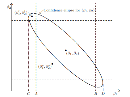
All students of econometrics are familiar with $\boldsymbol{t}$ statistics for testing hypotheses about a single parameter and $\boldsymbol{F}$ statistics for testing hypotheses about several parameters jointly. If $\hat{\beta}{i}$ denotes the least squares estimate of the parameter $\beta{i}$, the $t$ statistic for testing the hypothesis that $\beta_{i}$ is equal to some specified value $\beta_{0 i}$ is simply expression (3.12), that is, $\hat{\beta}{i}-\beta{0 i}$ divided by the estimated standard error of $\hat{\beta}_{i}$. If $\hat{\beta}$ denotes a set of unrestricted least squares estimates and $\overline{\boldsymbol{\beta}}$ denotes a set of estimates subject to $r$ distinct restrictions, then the $F$ statistic for testing those restrictions may be calculated as
$$
\frac{(\operatorname{SSR}(\overline{\boldsymbol{\beta}})-\operatorname{SSR}(\hat{\boldsymbol{\beta}})) / r}{\operatorname{SSR}(\hat{\boldsymbol{\beta}}) /(n-k)}=\frac{1}{r s^{2}}(\operatorname{SSR}(\overline{\boldsymbol{\beta}})-\operatorname{SSR}(\hat{\boldsymbol{\beta}}))
$$
Tests based on $t$ and $F$ statistics may be either exact or approximate. In the very special case referred to at the end of the last section, in which the regression model and the restrictions are both linear in the parameters, the regressors are (or can be treated as) fixed in repeated samples, and the error terms are normally and independently distributed, ordinary $t$ and $F$ statistics
actually are distributed in finite samples under the null hypotheses according to their namesake distributions. Although this case is not encountered nearly as often as one might hope, these results are sufficiently important that they are worth a separate section. Moreover, it is useful to keep the linear case firmly in mind when considering the case of nonlinear regression models.
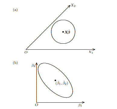
Consider the restricted model
$$
\boldsymbol{y}=\boldsymbol{X}{1} \beta{1}+\boldsymbol{u}
$$
and the unrestricted model
$$
\boldsymbol{y}=\boldsymbol{X}{1} \boldsymbol{\beta}{1}+\boldsymbol{X}{2} \boldsymbol{\beta}{2}+\boldsymbol{u}
$$
经济代写|计量经济学作业代写Econometrics代考|Hypothesis Testing in Nonlinear Regression Models
There are at least three different ways that we can derive test statistics for hypotheses about the parameters of nonlinear regression models. They are to utilize the Wald principle, the Lagrange multiplier principle, and the likelihood ratio principle. These yield what are often collectively referred to as the three “classical” test statistics. In this section, we introduce these three principles and show how they yield test statistics for hypotheses about $\boldsymbol{\beta}$ in nonlinear regression models (and implicitly in linear regression models as well, since linear models are simply a special case of nonlinear ones). The three principles are very widely applicable and will reappear in other contexts throughout the book. ${ }^{7}$ A formal treatment of these tests in the context of least squares will be provided in Chapter 5. They will be reintroduced in the context of maximum likelihood estimation in Chapter 8 , and a detailed treatment in that context will be provided in Chapter 13. Valuable referencer include Engle (1984) and Godfrey (1988), and an illuminating introductory discussion may be found in Buse (1982).
The Wald principle, which is due to Wald (1943), is to construct a test statistic based on unrestricted parameter estimates and an estimate of the unrestricted covariance matrix. If the hypothesis involves just one restriction, say that $\beta_{i}=\beta_{i}^{}$, then one can calculate the pseudo- $t$ statistic $$ \frac{\hat{\beta}{i}-\beta{i}^{}}{\hat{S}\left(\hat{\beta}{i}\right)} . $$ We refer to this as a “pseudo-t” statistic because it will not actually have the Student’s $t$ distribution with $n-k$ degrees of freedom in finite samples when $x{t}(\boldsymbol{\beta})$ is nonlinear in the parameters, $x_{t}(\boldsymbol{\beta})$ depends on lagged values of $y_{t}$, or the errors $u_{t}$ are not normally distributed. However, it will be asymptotically distributed as $N(0,1)$ under quite weak conditions (see Chapter 5 ), and its finite-sample distribution is frequently approximated quite well by $t(n-k)$.
In the more general case in which there are $r$ restrictions rather than just one to be tested, Wald tests make use of the fact that if $v$ is a random $r$-vector which is normally distributed with mean vector zero and covariance matrix $\boldsymbol{\Lambda}$, then the quadratic form
$$
\boldsymbol{v}^{\top} \boldsymbol{\Lambda}^{-1} \boldsymbol{v}
$$
must be distributed as $\chi^{2}(r)$. This result is proved in Appendix $\mathrm{B}$, and we used it in Sections $3.3$ and $3.5$ above.
To construct an asymptotic Wald test, then, we simply have to find a vector of random variables that should under the null hypothesis be asymptotically normally distributed with mean vector zero and a covariance matrix which we can estimate. For example, suppose that $\beta$ is subject to the $r(\leq k)$ linearly independent restrictions
$$
\boldsymbol{R} \boldsymbol{\beta}=\boldsymbol{r},
$$
计量经济学代考
经济代写|计量经济学作业代写Econometrics代考|Hypothesis Testing: Introduction
经济学家经常希望检验关于他们估计的回归模型的假设。这种假设通常采用对某些参数进行等式限制的形式。它们可能涉及测试单个参数是否具有特定值(例如,b2=1),两个参数是否以特定方式相关(例如,b3=2b4),是否是非线性限制,例如b1/b3=b2/b4成立,或者也许一整套线性和/或非线性限制成立。要测试的限制或一组限制确实成立的假设称为原假设,通常表示为H0. 限制不成立的模型通常称为备择假设,或有时称为维持假设,并且可以表示为H1. 术语“维持假设”反映了这样一个事实,即在统计检验中,只有零假设H0正在测试中。拒绝H0不以任何方式迫使我们接受H1,因为它不是H1我们正在测试。考虑如果 DGP 不是特殊情况会发生什么H1. 显然两者H0和H1那么将是错误的,并且很有可能测试H0会导致它的拒绝。其他测试很可能成功拒绝错误H1,但前提是它随后扮演了原假设的角色并找到了一些新的维持假设。
本书中讨论的所有假设检验都涉及生成检验统计量。一个测试统计,比如说吨, 是一个随机变量,其概率分布在原假设下准确或近似已知。然后我们看到观察值的可能性有多大吨根据那个概率分布,应该已经发生了。如果吨是一个很容易偶然发生的数字,那么我们没有证据反对原假设H0. 但是,如果它是一个很少偶然出现的数字,我们确实有证据反对 null,我们很可能决定拒绝它。
执行测试的经典方法是将一组可能的值除以吨分为两个区域,接受区域和拒绝区域(或临界区域)。如果吨落入接受区域,零假设被接受(或无论如何不被拒绝),而如果它落入拒绝区域,则被拒绝。5例如,如果吨已知有一个χ2分布,接受范围将包括所有价值吨cqual 或 lcsis 大于某个临界值,比如说C,然后拒绝区域将包含所有大于C.如果相反吨已知具有正态分布,那么对于双尾测试,接受区域将由所有绝对值组成吨小于或等于C. 因此,拒绝区域将包括
两部分,一部分包含的值大于C并且一部分包含的值小于−C.
检验的大小是当零假设为真时,检验统计量拒绝零假设的概率。让θ表示要测试的参数向量;θ0, 的值集θ满足H0; 和R,拒绝域。然后是测试的大小吨是
一种≡公关(吨∈R∣θ∈θ0)
经济代写|计量经济学作业代写Econometrics代考|Hypothesis Testing in Linear Regression Models
所有计量经济学的学生都熟悉吨用于检验关于单个参数的假设的统计数据和F用于联合检验几个参数的假设的统计量。如果b^一世表示参数的最小二乘估计b一世, 这吨用于检验假设的统计量b一世等于某个指定值b0一世是简单的表达式(3.12),即b^一世−b0一世除以估计的标准误差b^一世. 如果b^表示一组不受限制的最小二乘估计和b¯表示一组估计值r明显的限制,那么F测试这些限制的统计量可以计算为
(固态继电器(b¯)−固态继电器(b^))/r固态继电器(b^)/(n−ķ)=1rs2(固态继电器(b¯)−固态继电器(b^))
测试基于吨和F统计数据可以是精确的也可以是近似的。在上一节末尾提到的非常特殊的情况下,其中回归模型和限制在参数上都是线性的,回归量在重复样本中是(或可以被视为)固定的,并且误差项是正态且独立分布,普通吨和F统计数据
实际上根据它们的同名分布分布在零假设下的有限样本中。尽管这种情况并不像人们希望的那样经常遇到,但这些结果非常重要,值得单独讨论。此外,在考虑非线性回归模型的情况时,牢牢记住线性情况是有用的。
考虑受限模型
是=X1b1+在
和不受限制的模型
是=X1b1+X2b2+在
经济代写|计量经济学作业代写Econometrics代考|Hypothesis Testing in Nonlinear Regression Models
对于非线性回归模型参数的假设,我们至少可以通过三种不同的方式得出检验统计量。他们将利用沃尔德原理、拉格朗日乘数原理和似然比原理。这些产生了通常被统称为三个“经典”测试统计量的东西。在本节中,我们将介绍这三个原则,并展示它们如何产生关于以下假设的检验统计量b在非线性回归模型中(也隐含在线性回归模型中,因为线性模型只是非线性模型的一个特例)。这三个原则适用性非常广泛,并且将在本书的其他上下文中重新出现。7第 5 章将在最小二乘的背景下对这些检验进行正式处理。第 8 章将在最大似然估计的背景下重新介绍这些检验,第 13 章将提供在该背景下的详细处理。 有价值的参考资料包括 Engle (1984) 和 Godfrey (1988),并且可以在 Buse (1982) 中找到具有启发性的介绍性讨论。
Wald 原理源于 Wald (1943),它是基于无限制参数估计和无限制协方差矩阵的估计构建检验统计量。如果假设只涉及一个限制,那么说b一世=b一世,那么可以计算出伪吨统计b^一世−b一世小号^(b^一世).我们将其称为“伪 t”统计量,因为它实际上没有学生的吨分布与n−ķ有限样本中的自由度X吨(b)参数是非线性的,X吨(b)取决于滞后值是吨,或错误在吨不是正态分布的。但是,它将渐近分布为ñ(0,1)在相当弱的条件下(见第 5 章),它的有限样本分布通常很好地近似为吨(n−ķ).
在更一般的情况下,有r限制而不仅仅是一个要测试的限制,Wald 测试利用了这样一个事实,即如果在是随机的r- 正态分布的向量,均值向量为零和协方差矩阵Λ,然后是二次形式
在⊤Λ−1在
必须分发为χ2(r). 这个结果在附录中得到证明乙, 我们在 Sections 中使用它3.3和3.5多于。
然后,为了构建渐近 Wald 检验,我们只需找到一个随机变量向量,该向量在原假设下应该是渐近正态分布的,均值向量为零和一个我们可以估计的协方差矩阵。例如,假设b受制于r(≤ķ)线性独立限制
Rb=r,

统计代写请认准statistics-lab™. statistics-lab™为您的留学生涯保驾护航。
随机过程代考
在概率论概念中,随机过程是随机变量的集合。 若一随机系统的样本点是随机函数,则称此函数为样本函数,这一随机系统全部样本函数的集合是一个随机过程。 实际应用中,样本函数的一般定义在时间域或者空间域。 随机过程的实例如股票和汇率的波动、语音信号、视频信号、体温的变化,随机运动如布朗运动、随机徘徊等等。
贝叶斯方法代考
贝叶斯统计概念及数据分析表示使用概率陈述回答有关未知参数的研究问题以及统计范式。后验分布包括关于参数的先验分布,和基于观测数据提供关于参数的信息似然模型。根据选择的先验分布和似然模型,后验分布可以解析或近似,例如,马尔科夫链蒙特卡罗 (MCMC) 方法之一。贝叶斯统计概念及数据分析使用后验分布来形成模型参数的各种摘要,包括点估计,如后验平均值、中位数、百分位数和称为可信区间的区间估计。此外,所有关于模型参数的统计检验都可以表示为基于估计后验分布的概率报表。
广义线性模型代考
广义线性模型(GLM)归属统计学领域,是一种应用灵活的线性回归模型。该模型允许因变量的偏差分布有除了正态分布之外的其它分布。
statistics-lab作为专业的留学生服务机构,多年来已为美国、英国、加拿大、澳洲等留学热门地的学生提供专业的学术服务,包括但不限于Essay代写,Assignment代写,Dissertation代写,Report代写,小组作业代写,Proposal代写,Paper代写,Presentation代写,计算机作业代写,论文修改和润色,网课代做,exam代考等等。写作范围涵盖高中,本科,研究生等海外留学全阶段,辐射金融,经济学,会计学,审计学,管理学等全球99%专业科目。写作团队既有专业英语母语作者,也有海外名校硕博留学生,每位写作老师都拥有过硬的语言能力,专业的学科背景和学术写作经验。我们承诺100%原创,100%专业,100%准时,100%满意。
机器学习代写
随着AI的大潮到来,Machine Learning逐渐成为一个新的学习热点。同时与传统CS相比,Machine Learning在其他领域也有着广泛的应用,因此这门学科成为不仅折磨CS专业同学的“小恶魔”,也是折磨生物、化学、统计等其他学科留学生的“大魔王”。学习Machine learning的一大绊脚石在于使用语言众多,跨学科范围广,所以学习起来尤其困难。但是不管你在学习Machine Learning时遇到任何难题,StudyGate专业导师团队都能为你轻松解决。
多元统计分析代考
基础数据: $N$ 个样本, $P$ 个变量数的单样本,组成的横列的数据表
变量定性: 分类和顺序;变量定量:数值
数学公式的角度分为: 因变量与自变量
时间序列分析代写
随机过程,是依赖于参数的一组随机变量的全体,参数通常是时间。 随机变量是随机现象的数量表现,其时间序列是一组按照时间发生先后顺序进行排列的数据点序列。通常一组时间序列的时间间隔为一恒定值(如1秒,5分钟,12小时,7天,1年),因此时间序列可以作为离散时间数据进行分析处理。研究时间序列数据的意义在于现实中,往往需要研究某个事物其随时间发展变化的规律。这就需要通过研究该事物过去发展的历史记录,以得到其自身发展的规律。
回归分析代写
多元回归分析渐进(Multiple Regression Analysis Asymptotics)属于计量经济学领域,主要是一种数学上的统计分析方法,可以分析复杂情况下各影响因素的数学关系,在自然科学、社会和经济学等多个领域内应用广泛。
MATLAB代写
MATLAB 是一种用于技术计算的高性能语言。它将计算、可视化和编程集成在一个易于使用的环境中,其中问题和解决方案以熟悉的数学符号表示。典型用途包括:数学和计算算法开发建模、仿真和原型制作数据分析、探索和可视化科学和工程图形应用程序开发,包括图形用户界面构建MATLAB 是一个交互式系统,其基本数据元素是一个不需要维度的数组。这使您可以解决许多技术计算问题,尤其是那些具有矩阵和向量公式的问题,而只需用 C 或 Fortran 等标量非交互式语言编写程序所需的时间的一小部分。MATLAB 名称代表矩阵实验室。MATLAB 最初的编写目的是提供对由 LINPACK 和 EISPACK 项目开发的矩阵软件的轻松访问,这两个项目共同代表了矩阵计算软件的最新技术。MATLAB 经过多年的发展,得到了许多用户的投入。在大学环境中,它是数学、工程和科学入门和高级课程的标准教学工具。在工业领域,MATLAB 是高效研究、开发和分析的首选工具。MATLAB 具有一系列称为工具箱的特定于应用程序的解决方案。对于大多数 MATLAB 用户来说非常重要,工具箱允许您学习和应用专业技术。工具箱是 MATLAB 函数(M 文件)的综合集合,可扩展 MATLAB 环境以解决特定类别的问题。可用工具箱的领域包括信号处理、控制系统、神经网络、模糊逻辑、小波、仿真等。