如果你也在 怎样代写计量经济学Econometrics这个学科遇到相关的难题,请随时右上角联系我们的24/7代写客服。
计量经济学是将统计方法应用于经济数据,以赋予经济关系以经验内容。
statistics-lab™ 为您的留学生涯保驾护航 在代写计量经济学Econometrics方面已经树立了自己的口碑, 保证靠谱, 高质且原创的统计Statistics代写服务。我们的专家在代写计量经济学Econometrics代写方面经验极为丰富,各种代写计量经济学Econometrics相关的作业也就用不着说。
我们提供的计量经济学Econometrics及其相关学科的代写,服务范围广, 其中包括但不限于:
- Statistical Inference 统计推断
- Statistical Computing 统计计算
- Advanced Probability Theory 高等楖率论
- Advanced Mathematical Statistics 高等数理统计学
- (Generalized) Linear Models 广义线性模型
- Statistical Machine Learning 统计机器学习
- Longitudinal Data Analysis 纵向数据分析
- Foundations of Data Science 数据科学基础
- Statistical Inference 统计推断
- Statistical Computing 统计计算
- Advanced Probability Theory 高等楖率论
- Advanced Mathematical Statistics 高等数理统计学
- (Generalized) Linear Models 广义线性模型
- Statistical Machine Learning 统计机器学习
- Longitudinal Data Analysis 纵向数据分析
- Foundations of Data Science 数据科学基础
经济代写|计量经济学作业代写Econometrics代考|Restrictions and Pretest Estimators
In the preceding three sections, we have discussed hypothesis testing at some length, but we have not said anything about one of the principal reasons for imposing and testing restrictions. In many cases, restrictions are not implied by any economic theory but are imposed by the investigator in the hope that a restricted model will be easier to estimate and will yield more efficient estimates than an unrestricted model. Tests of this sort of restriction include DWH tests (Chapter 7), tests for serial correlation (Chapter 10), common factor restriction tests (Chapter 10), tests for structural change (Chapter 11), and tests on the length of a distributed lag (Chapter 19). In these and many other cases, restrictions are tested in order to decide which model to use as a basis for inference about the parameters of interest and to weed out models that appear to be incompatible with the data. However, because estimation and testing are based on the same data, the properties of the final estimates may be very difficult to analyze. This is the problem of pretesting.
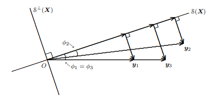
For simplicity, we will in this section consider only the case of linear regression models with fixed regressors, some coefficients of which are subject to zero restrictions. The restricted model will be (3.18), in which $\boldsymbol{y}$ is regressed on an $n \times(k-r)$ matrix $\boldsymbol{X}{1}$, and the unrestricted model will be (3.19), in which $\boldsymbol{y}$ is regressed on $\boldsymbol{X}{1}$ and an $n \times r$ matrix $\boldsymbol{X}{2}$. The OLS estimates of the parameters of the restricted model are $$ \overline{\boldsymbol{\beta}}{1}=\left(\boldsymbol{X}{1}^{\top} \boldsymbol{X}{1}\right)^{-1} \boldsymbol{X}{1}^{\top} \boldsymbol{y} $$ The OLS estimates of these same parameters in the unrestricted model can easily he found hy using, the FWT. Thenrem. They are $$ \hat{\boldsymbol{\beta}}{1}=\left(\boldsymbol{X}{1}^{\top} \boldsymbol{M}{2} \boldsymbol{X}{1}\right)^{-1} \boldsymbol{X}{1}^{\top} \boldsymbol{M}{2} \boldsymbol{y} $$ where $\boldsymbol{M}{2}$ denotes the matrix that projects orthogonally onto $\mathcal{S}^{\perp}\left(\boldsymbol{X}{2}\right)$. It is natural to ask how well the estimators $\overline{\boldsymbol{\beta}}{1}$ and $\hat{\boldsymbol{\beta}}{1}$ perform relative to each other. If the data are actually generated by the DGP (3.22), which is a special case of the restricted model, they are evidently both unbiased. However, as we will demonstrate in a moment, the restricted estimator $\overline{\boldsymbol{\beta}}{1}$ is more efficient than the unrestricted estimator $\hat{\beta}{1}$. One estimator is said to be more efficient than another if the covariance matrix of the inefficient estimator minus the covariance matrix of the efficient one is a positive semidefinite matrix; see Section 5.5. If $\overline{\boldsymbol{\beta}}{1}$ is more efficient than $\hat{\boldsymbol{\beta}}{1}$ in this sense, then any linear combination of the elements of $\bar{\beta}{1}$ must have variance no larger than the corresponding linear combination of the elements of $\hat{\beta}_{1}$.
The proof that $\overline{\boldsymbol{\beta}}{1}$ is more efficient than $\hat{\boldsymbol{\beta}}{1}$ under the DGP (3.22) is very simple. The difference between the covariance matrices of $\hat{\boldsymbol{\beta}}{1}$ and $\overline{\boldsymbol{\beta}}{1}$ is
$$
\sigma_{0}^{2}\left(\boldsymbol{X}{1}^{\top} \boldsymbol{M}{2} \boldsymbol{X}{1}\right)^{-1}-\sigma{0}^{2}\left(\boldsymbol{X}{1}^{\top} \boldsymbol{X}{1}\right)^{-1}
$$
经济代写|计量经济学作业代写Econometrics代考|pretest estimator
Pretest estimators are used all the time. Whenever we test some aspect of a model’s specification and then decide, on the basis of the test results, what version of the model to estimate or what estimation method to use, we are employing a pretest estimator. Unfortunately, the properties of pretest estimators are, in practice, very difficult to know. The problems can been from the example we have been studying. Suppose the restrictions hold. Then the estimator we would like to use is the restricted estimator, $\overline{\boldsymbol{\beta}}{1}$. But, $\alpha \%$ of the time, the $F$ test will incorrectly reject the null hypothesis and $\beta{1}$ will be equal to the unrestricted estimator $\hat{\boldsymbol{\beta}}{1}$ instead. Thus $\check{\boldsymbol{\beta}}{1}$ must be less efficient than $\overline{\boldsymbol{\beta}}{1}$ when the restrictions do in fact hold. Moreover, since the estimated covariance matrix reported by the regression package will not take the pretesting into account, inferences about $\boldsymbol{\beta}{1}$ may be misleading.
On the other hand, when the restrictions do not hold, we may or may not want to use the unrestricted estimator $\hat{\beta}{1}$. Depending on how much power the $F$ test has, $\check{\boldsymbol{\beta}}{1}$ will sometimes be equal to $\overline{\boldsymbol{\beta}}{1}$ and sometimes be equal to $\hat{\boldsymbol{\beta}}{1}$. It will certainly not be unbiased, because $\overline{\boldsymbol{\beta}}{1}$ is not unbiased, and it may be more or less efficient (in the sense of mean squared error) than the unrestricted estimator. Inferences about $\check{\boldsymbol{\beta}}{1}$ based on the usual estimated OLS covariance matrix for whichever of $\overline{\boldsymbol{\beta}}{1}$ and $\hat{\boldsymbol{\beta}}{1}$ it turns out to be equal to may be misleading, because they fail to take into account the pretesting that occurred previously.
In practice, there is often not very much that we can do about the problems caused by pretesting, except to recognize that pretesting adds an additional element of uncertainty to most problems of statistical inference. Since $\alpha$, the level of the preliminary test, will affect the properties of $\boldsymbol{\beta}_{1}$, it may be worthwhile to try using different values of $\alpha$. Conventional significance levels such as $.05$ are certainly not optimal in general, and there is a literature on how to choose better ones in specific cases; see, for example, Toyoda and Wallace (1976). However, real pretesting problems are much more complicated than the one we have discussed as an example or the ones that have been studied in the literature. Every time one subjects a model to any sort of test, the result of that test may affect the form of the final model, and the implied pretest estimator therefore becomes even more complicated. It is hard to see how this can be analyzed formally.
经济代写|计量经济学作业代写Econometrics代考|Conclusion
This chapter has provided an introduction to several important topics: estimation of covariance matrices for NLS estimates, the use of such covariance matrix estimates for constructing confidence intervals, basic ideas of hypothesis testing, the justification for testing linear restrictions on linear regression models by means of $t$ and $F$ tests, the three classical principles of hypothesis testing and their application to nonlinear regression models, and pretesting. At a number of points we were forced to be a little vague and to refer to results on the asymptotic properties of nonlinear least squares estimates that we have not yet proved. Proving those results will be the object of the next two chapters. Chapter 4 discusses the basic ideas of asymptotic analysis, including consistency, asymptotic normality, central limit theorems, laws of large numbers, and the use of “big- $O$ ” and “little-o” notation. Chapter 5 then uses these concepts to prove the consistency and asymptotic normality of nonlinear least squares estimates of univariate nonlinear regression models and to derive the asymptotic distributions of the test statistics discussed in this chapter. It also proves a number of related asymptotic results that will be useful later on.
计量经济学代考
经济代写|计量经济学作业代写Econometrics代考|Restrictions and Pretest Estimators
在前面的三节中,我们已经详细讨论了假设检验,但我们没有提及施加和检验限制的主要原因之一。在许多情况下,任何经济理论都没有暗示限制,而是由研究人员强加的,希望限制模型比无限制模型更容易估计并产生更有效的估计。这种限制的检验包括 DWH 检验(第 7 章)、序列相关检验(第 10 章)、公因子限制检验(第 10 章)、结构变化检验(第 11 章)和分布滞后长度检验(第 19 章)。在这些和许多其他情况下,测试限制是为了决定使用哪个模型作为推断感兴趣参数的基础,并剔除看起来与数据不兼容的模型。但是,由于估计和测试基于相同的数据,最终估计的属性可能很难分析。这就是预测试的问题。
为简单起见,我们将在本节中仅考虑具有固定回归量的线性回归模型的情况,其中一些系数受到零限制。受限模型将是 (3.18),其中是回归到一个n×(ķ−r)矩阵X1, 不受限制的模型将是 (3.19), 其中是回归于X1和n×r矩阵X2. 受限模型参数的 OLS 估计为b¯1=(X1⊤X1)−1X1⊤是使用 FWT 可以很容易地发现无限制模型中这些相同参数的 OLS 估计。恩雷姆。他们是b^1=(X1⊤米2X1)−1X1⊤米2是在哪里米2表示正交投影到的矩阵小号⊥(X2). 很自然地要问估算器的效果如何b¯1和b^1相对执行。如果数据实际上是由 DGP (3.22) 生成的,这是受限模型的一个特例,它们显然都是无偏的。然而,正如我们稍后将展示的,受限估计量b¯1比无限制估计器更有效b^1. 如果低效估计量的协方差矩阵减去有效估计量的协方差矩阵是半正定矩阵,则称一个估计量比另一种更有效;见第 5.5 节。如果b¯1比b^1在这个意义上,那么任何元素的线性组合b¯1方差必须不大于元素的相应线性组合b^1.
证明b¯1比b^1DGP(3.22)下很简单。协方差矩阵之间的差异b^1和b¯1是
σ02(X1⊤米2X1)−1−σ02(X1⊤X1)−1
经济代写|计量经济学作业代写Econometrics代考|pretest estimator
预测试估计器一直在使用。每当我们测试模型规范的某些方面,然后根据测试结果决定要估计的模型版本或使用的估计方法时,我们都在使用预测试估计器。不幸的是,在实践中,预测估计量的性质很难知道。这些问题可能来自我们一直在研究的例子。假设限制成立。那么我们想要使用的估计器是受限估计器,b¯1. 但,一种%当时,F测试将错误地拒绝原假设并且b1将等于无限制估计量b^1反而。因此bˇ1效率必须低于b¯1当限制确实成立时。此外,由于回归包报告的估计协方差矩阵不会考虑预测试,因此关于b1可能会产生误导。
另一方面,当限制不成立时,我们可能想也可能不想使用不受限制的估计量b^1. 取决于功率多少F测试有,bˇ1有时会等于b¯1有时等于b^1. 它肯定不会不偏不倚,因为b¯1不是无偏的,并且它可能比无限制估计量更有效(在均方误差的意义上)。关于的推论bˇ1基于通常估计的 OLS 协方差矩阵b¯1和b^1事实证明等于 可能具有误导性,因为它们没有考虑到之前发生的预测试。
在实践中,对于由预测试引起的问题,我们通常无能为力,除了认识到预测试给大多数统计推断问题增加了额外的不确定因素。自从一种,初试的高低,会影响属性b1,可能值得尝试使用不同的值一种. 传统的显着性水平,例如.05通常肯定不是最优的,并且有关于如何在特定情况下选择更好的文献;例如,参见 Toyoda 和 Wallace (1976)。然而,真正的预测试问题比我们作为例子讨论的问题或文献中研究过的问题要复杂得多。每次对模型进行任何类型的测试时,该测试的结果都可能影响最终模型的形式,因此隐含的预测试估计量变得更加复杂。很难看到如何正式分析这一点。
经济代写|计量经济学作业代写Econometrics代考|Conclusion
本章介绍了几个重要主题:NLS 估计的协方差矩阵估计、使用协方差矩阵估计构建置信区间、假设检验的基本思想、通过吨和F测试,假设检验的三个经典原则及其在非线性回归模型中的应用,以及预测试。在许多方面,我们被迫有点模糊,并参考我们尚未证明的非线性最小二乘估计的渐近性质的结果。证明这些结果将是接下来两章的目标。第 4 章讨论了渐近分析的基本思想,包括一致性、渐近正态性、中心极限定理、大数定律,以及“big-这”和“little-o”符号。然后第 5 章使用这些概念来证明单变量非线性回归模型的非线性最小二乘估计的一致性和渐近正态性,并推导出本章讨论的检验统计量的渐近分布。它还证明了一些相关的渐近结果,这些结果将在以后有用。

统计代写请认准statistics-lab™. statistics-lab™为您的留学生涯保驾护航。
随机过程代考
在概率论概念中,随机过程是随机变量的集合。 若一随机系统的样本点是随机函数,则称此函数为样本函数,这一随机系统全部样本函数的集合是一个随机过程。 实际应用中,样本函数的一般定义在时间域或者空间域。 随机过程的实例如股票和汇率的波动、语音信号、视频信号、体温的变化,随机运动如布朗运动、随机徘徊等等。
贝叶斯方法代考
贝叶斯统计概念及数据分析表示使用概率陈述回答有关未知参数的研究问题以及统计范式。后验分布包括关于参数的先验分布,和基于观测数据提供关于参数的信息似然模型。根据选择的先验分布和似然模型,后验分布可以解析或近似,例如,马尔科夫链蒙特卡罗 (MCMC) 方法之一。贝叶斯统计概念及数据分析使用后验分布来形成模型参数的各种摘要,包括点估计,如后验平均值、中位数、百分位数和称为可信区间的区间估计。此外,所有关于模型参数的统计检验都可以表示为基于估计后验分布的概率报表。
广义线性模型代考
广义线性模型(GLM)归属统计学领域,是一种应用灵活的线性回归模型。该模型允许因变量的偏差分布有除了正态分布之外的其它分布。
statistics-lab作为专业的留学生服务机构,多年来已为美国、英国、加拿大、澳洲等留学热门地的学生提供专业的学术服务,包括但不限于Essay代写,Assignment代写,Dissertation代写,Report代写,小组作业代写,Proposal代写,Paper代写,Presentation代写,计算机作业代写,论文修改和润色,网课代做,exam代考等等。写作范围涵盖高中,本科,研究生等海外留学全阶段,辐射金融,经济学,会计学,审计学,管理学等全球99%专业科目。写作团队既有专业英语母语作者,也有海外名校硕博留学生,每位写作老师都拥有过硬的语言能力,专业的学科背景和学术写作经验。我们承诺100%原创,100%专业,100%准时,100%满意。
机器学习代写
随着AI的大潮到来,Machine Learning逐渐成为一个新的学习热点。同时与传统CS相比,Machine Learning在其他领域也有着广泛的应用,因此这门学科成为不仅折磨CS专业同学的“小恶魔”,也是折磨生物、化学、统计等其他学科留学生的“大魔王”。学习Machine learning的一大绊脚石在于使用语言众多,跨学科范围广,所以学习起来尤其困难。但是不管你在学习Machine Learning时遇到任何难题,StudyGate专业导师团队都能为你轻松解决。
多元统计分析代考
基础数据: $N$ 个样本, $P$ 个变量数的单样本,组成的横列的数据表
变量定性: 分类和顺序;变量定量:数值
数学公式的角度分为: 因变量与自变量
时间序列分析代写
随机过程,是依赖于参数的一组随机变量的全体,参数通常是时间。 随机变量是随机现象的数量表现,其时间序列是一组按照时间发生先后顺序进行排列的数据点序列。通常一组时间序列的时间间隔为一恒定值(如1秒,5分钟,12小时,7天,1年),因此时间序列可以作为离散时间数据进行分析处理。研究时间序列数据的意义在于现实中,往往需要研究某个事物其随时间发展变化的规律。这就需要通过研究该事物过去发展的历史记录,以得到其自身发展的规律。
回归分析代写
多元回归分析渐进(Multiple Regression Analysis Asymptotics)属于计量经济学领域,主要是一种数学上的统计分析方法,可以分析复杂情况下各影响因素的数学关系,在自然科学、社会和经济学等多个领域内应用广泛。
MATLAB代写
MATLAB 是一种用于技术计算的高性能语言。它将计算、可视化和编程集成在一个易于使用的环境中,其中问题和解决方案以熟悉的数学符号表示。典型用途包括:数学和计算算法开发建模、仿真和原型制作数据分析、探索和可视化科学和工程图形应用程序开发,包括图形用户界面构建MATLAB 是一个交互式系统,其基本数据元素是一个不需要维度的数组。这使您可以解决许多技术计算问题,尤其是那些具有矩阵和向量公式的问题,而只需用 C 或 Fortran 等标量非交互式语言编写程序所需的时间的一小部分。MATLAB 名称代表矩阵实验室。MATLAB 最初的编写目的是提供对由 LINPACK 和 EISPACK 项目开发的矩阵软件的轻松访问,这两个项目共同代表了矩阵计算软件的最新技术。MATLAB 经过多年的发展,得到了许多用户的投入。在大学环境中,它是数学、工程和科学入门和高级课程的标准教学工具。在工业领域,MATLAB 是高效研究、开发和分析的首选工具。MATLAB 具有一系列称为工具箱的特定于应用程序的解决方案。对于大多数 MATLAB 用户来说非常重要,工具箱允许您学习和应用专业技术。工具箱是 MATLAB 函数(M 文件)的综合集合,可扩展 MATLAB 环境以解决特定类别的问题。可用工具箱的领域包括信号处理、控制系统、神经网络、模糊逻辑、小波、仿真等。