如果你也在 怎样代写主成分分析Principal Component Analysis这个学科遇到相关的难题,请随时右上角联系我们的24/7代写客服。
主成分分析(PCA)是计算主成分并使用它们对数据进行基础改变的过程,有时只使用前几个主成分,而忽略其余部分。
statistics-lab™ 为您的留学生涯保驾护航 在代写主成分分析Principal Component Analysis方面已经树立了自己的口碑, 保证靠谱, 高质且原创的统计Statistics代写服务。我们的专家在代写主成分分析Principal Component Analysis代写方面经验极为丰富,各种代写主成分分析Principal Component Analysis相关的作业也就用不着说。
我们提供的主成分分析Principal Component Analysis及其相关学科的代写,服务范围广, 其中包括但不限于:
- Statistical Inference 统计推断
- Statistical Computing 统计计算
- Advanced Probability Theory 高等概率论
- Advanced Mathematical Statistics 高等数理统计学
- (Generalized) Linear Models 广义线性模型
- Statistical Machine Learning 统计机器学习
- Longitudinal Data Analysis 纵向数据分析
- Foundations of Data Science 数据科学基础
统计代写|主成分分析代写Principal Component Analysis代考|Missing Not at Random
When the distribution of the missing data indicator depends on the unobserved data, after conditioning on the observed data, i.e. when
$$
\operatorname{Pr}\left(\mathbf{m}{i} \mid \mathbf{z}{i}, \mathbf{x}{i}\right) \neq \operatorname{Pr}\left(\mathbf{m}{i} \mid \mathbf{x}_{i}\right)
$$
then the missing data are said to be missing not at random. This setting is the most general of all.
In the MNAR scenario the missingness indicator is assumed to be related with unmeasured predictors and/or the unobserved response, even conditionally on the observed data. MNAR data are also referred to as informative since the missing values contain information about the MNAR mechanism itself.
It should be stressed that, if the true mechanism is MNAR, simple CC analyses or naïve imputation methods inevitably produce biased results. The extent and direction of this bias is unpredictable, and even relatively small fractions of missing values might lead to a large bias.
There are different approaches to the treatment of this kind of missing data. Modelbased procedures are most commonly adopted. These aim at modeling the joint distribution of the measurement process and the dropout process, by specifying a missing data model (MDM). The MDM must take into account the residual dependence between the missingness indicator and the unobserved response. Below, we summarize the three main approaches.
- Pattern-mixture models. The joint distribution of $\mathbf{y}{i}$ and $\mathbf{m}{i}$ is factorized as
$$
\operatorname{Pr}\left(\mathbf{y}{i}, \mathbf{m}{i}\right)=\operatorname{Pr}\left(\mathbf{y}{i} \mid \mathbf{m}{i}\right) \operatorname{Pr}\left(\mathbf{m}{i}\right) $$ This approach involves formulating separate submodels $\operatorname{Pr}\left(\mathbf{y}{i} \mid \mathbf{m}{i}\right)$ for each possible configuration of $\mathbf{m}{i}$, or, at least, for each observed configuration. This is appealing for studies where the main objective is to compare the response distribution in subgroups with possibly different missing value patterns. On the other hand, its specification can be cumbersome, while its interpretation at the population level may become difficult. - Selection models. The joint distribution of $\mathbf{y}{i}$ and $\mathbf{m}{i}$ is factorized as
$$
\operatorname{Pr}\left(\mathbf{y}{i}, \mathbf{m}{i}\right)=\operatorname{Pr}\left(\mathbf{m}{i} \mid \mathbf{y}{i}\right) \operatorname{Pr}\left(\mathbf{y}{i}\right) $$ This approach involves an explicit model to handle the distribution of the missing data process given the measurement mechanism. If correctly specified, the model for $\mathbf{y}{i}$ is estimated without bias and its interpretation is not compromised.
统计代写|主成分分析代写Principal Component Analysis代考|Methods to Handle Missing Data in Principal
In this section, we discuss selected missing data methods in PCA, some of which are relatively recent at the time of writing. PCA, originally introduced by Karl Pearson [34], is arguably one the most popular multivariate analysis techniques. It is often described as a tool for dimensionality reduction. Some authors consider PCA as a descriptive method, which needs not be based on distributional assumptions, whereas others provide probabilistic justifications in relation to sampling errors (see for example [20] or [21] for alternative interpretations of the PCA model). It is not our purpose to get embroiled in this discussion; here we take a probabilistic view as it is an essential framework for a statistical treatment of the missing data problem.
There are basically two main approaches where sampling comes into play: fixed and random effects PCA. (The random-effects approach can be formulated in either a frequentist or a Bayesian framework. We focus on the former, while more details on the latter can be found in [21]). In the fixed-effects approach, individuals are of direct interest. Therefore, individual-specific scores are parameters to be estimated. In symbols, the fixed-effects PCA model is given by
$$
\mathbf{y}{i}=\mu+\mathbf{W b}{i}+\varepsilon_{i}, \quad i=1, \ldots, n
$$
where $\mu=\left(\mu_{1}, \mu_{2}, \ldots, \mu_{p}\right)^{\mathrm{T}}$ is the vector with the mean of each variable, $\mathbf{b}{i}=$ $\left(b{i 1}, b_{i 2}, \ldots, b_{i q}\right)^{\mathrm{T}}$ is the $i$ th row vector of fixed scores and $\mathbf{W}$ is a $p \times q$ matrix of unknown loadings with elements $w_{j h}, j=1, \ldots, p, h=1, \ldots, q$, with $q \leq p$. The error is assumed to be zero-centered Gaussian with homoscedastic variance, $\varepsilon_{i} \sim N\left(\mathbf{0}, \psi \mathbf{I}{p}\right)$, where $\psi$ is a positive scalar. Model (6)’s parameter, $\boldsymbol{\theta}=\left(\boldsymbol{\mu}, \mathbf{W}, \psi, \mathbf{b}{1}, \mathbf{b}{2}, \ldots, \mathbf{b}{n}\right)$, can be estimated via maximum likelihood (or, equivalently, least squares) estimation (MLE). A downside of this approach is that the dimension of $\theta$ increases with the sample size.
The random-effects specification of the probabilistic representation of PCA $[38$, $42]$ is given by the model
$$
\mathbf{y}{i}=\mu+\mathbf{W u}{i}+\boldsymbol{\varepsilon}{i}, \quad i=1, \ldots, n $$ where $\mathbf{u}{i}=\left(u_{i 1}, u_{i 2}, \ldots, u_{i q}\right)^{\top}$ is the $i$ th row vector of latent scores and $\mathbf{W}$ is, as above, a matrix of unknown loadings. Furthermore, it is assumed that $\mathbf{u}$ is stochastically independent from $\varepsilon$. Conventionally, $\mathbf{u}{i} \sim N\left(0, \mathbf{I}{q}\right)$. If in addition the error is assumed to be zero-centered Gaussian with covariance matrix $\Psi, \varepsilon_{i} \sim N(0, \Psi)$, we obtain the multivariate normal distribution $\mathbf{y}{i} \sim N(\boldsymbol{\mu}, \mathbf{C}), \mathbf{C}=\mathbf{W} \mathbf{W}^{\top}+\boldsymbol{\Psi}$. We also assume that $\Psi=\psi \mathbf{I}{p}$, so that the elements of $\mathbf{y}{i}$ are conditionally independent, given $\mathbf{u}{i}$. The parameter $\mu=\left(\mu_{1}, \mu_{2}, \ldots, \mu_{p}\right)^{\top}$ allows for a location-shift fixed effect.
统计代写|主成分分析代写Principal Component Analysis代考|Multiple Imputation
As mentioned before, single imputation methods treat imputed missing values as fixed (known). This means that the uncertainty related to the missing values is ignored, which generally leads to deflated standard errors. Josse et al. [23] proposed to deal with this issue by first performing a residual bootstrap procedure to obtain $B$ estimates of the PPCA parameters and then generate $B$ data matrices, each completed with samples from the predictive distribution of the missing values conditional on the observed values and the corresponding bootstrapped parameter set. More formally, one can proceed as follows:
- obtain an initial estimate $\hat{\mu}, \hat{\mathbf{W}}, \hat{\mathbf{b}}_{i}, i=1, \ldots, n$, of the parameters in model (6) (e.g., via EM-PCA estimation). Reconstruct the data $\hat{\mathbf{Y}}$ with the first $q$ dimensions and calculate $\mathbf{R}=\mathbf{Y}-\hat{\mathbf{Y}}$, where the $n \times p$ matrix $\mathbf{R}$ of residuals has missing entries corresponding to those of $\mathbf{Y}$;
- draw $B$ random samples from the non-missing rows of $\mathbf{R}$. Denote each replicate by $\mathbf{R}_{b}^{*}, b=1, \ldots, B$;
- calculate $\mathbf{Y}{b}^{}=\hat{\mathbf{Y}}+\mathbf{R}{b}^{}, b=1, \ldots, B$ and estimate the PPCA parameters $\hat{\boldsymbol{\mu}}{b}^{}$, $\hat{\mathbf{W}}{b}^{}, \hat{\mathbf{b}}{b, i}^{}, i=1, \ldots, n$, from $\mathbf{Y}{b}^{}, b=1, \ldots, B ;$
- for $\left{i: s_{i}>0\right}$, calculate $\mathbf{y}{b, i}^{}=\hat{\boldsymbol{\mu}}{b}^{}+\hat{\mathbf{W}}{b}^{} \hat{\mathbf{b}}{b, i}^{}+\mathbf{r}^{}$, where $\mathbf{r}^{}$ is a newly sampled residual from $\mathbf{R}$. Complete the vector $\mathbf{y}{i}$ with $\mathbf{y}{b, i}^{*}$ to obtain the $b$ th complete data matrix $\mathbf{Y}_{b}, b=1, \ldots, B$.
There are several ways to obtain bootstrapped residuals. One approach is to draw a sample with replacement from the entries of the matrix $\mathbf{R}$. Another approach, recommended by [21], is to sample the residuals from a zero-centered Gaussian with variance estimated from the non-missing entries of $\mathbf{R}$. Improved results might be obtained with corrected residuals (e.g., leave-one-out residuals).
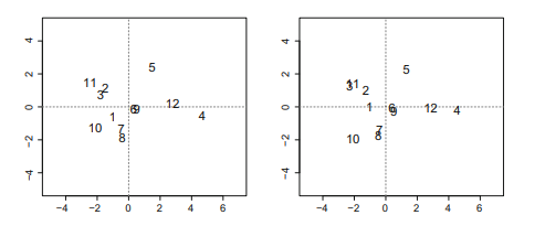
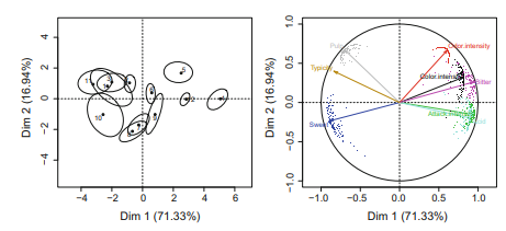
Once $B$ complete data matrices have been generated, the simplest analytic approach is to carry out a PPCA on each $\mathbf{Y}_{b}$, and then calculate the average of the $B$ sets of parameters. A multiple imputation PPCA of the Orange data set is given in R code 3.4. Our example is based on $B=100$ replicates, with $q=2$. The individuals and variables maps obtained from average scores and loadings are plotted in Fig. 2. As compared to the complete case PCA and the single imputation EM-PCA (Table 1), the multiple imputation PCA produced noticeably different estimates of $\hat{\mathbf{W}}$, especially for the second principal axis (R code $3.4$ ). The uncertainty due to the missing values is also shown in Fig. 2. For example, individual scores 1, 9, and 10 showed more total variability, as given by the area of the ellipses, and more variability along the second axis, as reflected in the eccentricity of the ellipses. The uncertainty was greater for sweetness, color intensity, and bitterness, and, as in the case of the individual scores, it was more prominent in relation to the second axis.
主成分分析代考
统计代写|主成分分析代写Principal Component Analysis代考|Missing Not at Random
当缺失数据指标的分布取决于未观察到的数据时,在对观察到的数据进行调节后,即当
公关(米一世∣和一世,X一世)≠公关(米一世∣X一世)
那么缺失的数据被称为不是随机缺失的。这个设置是最通用的。
在 MNAR 场景中,假设缺失指标与未测量的预测变量和/或未观察到的响应相关,甚至在观察数据的条件下也是如此。MNAR 数据也被称为信息性数据,因为缺失值包含有关 MNAR 机制本身的信息。
需要强调的是,如果真正的机制是 MNAR,简单的 CC 分析或朴素的插补方法不可避免地会产生有偏差的结果。这种偏差的程度和方向是不可预测的,即使是相对较小的缺失值也可能导致较大的偏差。
处理这种缺失数据有不同的方法。最常采用基于模型的程序。这些旨在通过指定缺失数据模型 (MDM) 对测量过程和退出过程的联合分布进行建模。MDM 必须考虑缺失指标和未观察到的响应之间的剩余依赖性。下面,我们总结了三种主要方法。
- 模式混合模型。联合分布是一世和米一世被分解为
公关(是一世,米一世)=公关(是一世∣米一世)公关(米一世)这种方法涉及制定单独的子模型公关(是一世∣米一世)对于每个可能的配置米一世,或者至少对于每个观察到的配置。这对于主要目标是比较可能具有不同缺失值模式的子组中的响应分布的研究很有吸引力。另一方面,它的规范可能很麻烦,而在人口水平上的解释可能会变得困难。 - 选择模型。联合分布是一世和米一世被分解为
公关(是一世,米一世)=公关(米一世∣是一世)公关(是一世)这种方法涉及一个显式模型来处理给定测量机制的缺失数据过程的分布。如果正确指定,模型为是一世估计没有偏见,它的解释没有妥协。
统计代写|主成分分析代写Principal Component Analysis代考|Methods to Handle Missing Data in Principal
在本节中,我们将讨论 PCA 中选定的缺失数据方法,其中一些在撰写本文时相对较新。PCA 最初由 Karl Pearson [34] 引入,可以说是最流行的多变量分析技术之一。它通常被描述为降维的工具。一些作者认为 PCA 是一种描述性方法,它不需要基于分布假设,而另一些作者则提供与抽样误差相关的概率论证明(参见例如 [20] 或 [21] 对 PCA 模型的替代解释)。卷入这个讨论不是我们的目的。在这里,我们采用概率观点,因为它是对缺失数据问题进行统计处理的基本框架。
抽样发挥作用的主要方法有两种:固定效应和随机效应 PCA。(随机效应方法可以在频率论或贝叶斯框架中制定。我们关注前者,而关于后者的更多细节可以在 [21] 中找到)。在固定效应方法中,个人是直接感兴趣的。因此,个人特定分数是要估计的参数。在符号中,固定效应 PCA 模型由下式给出
是一世=μ+在b一世+e一世,一世=1,…,n
在哪里μ=(μ1,μ2,…,μp)吨是每个变量均值的向量,b一世= (b一世1,b一世2,…,b一世q)吨是个一世固定分数的第行向量和在是一个p×q元素未知载荷矩阵在jH,j=1,…,p,H=1,…,q, 和q≤p. 假设误差是具有同方差方差的零中心高斯,e一世∼ñ(0,ψ我p), 在哪里ψ是一个正标量。模型(6)的参数,θ=(μ,在,ψ,b1,b2,…,bn),可以通过最大似然(或等效地,最小二乘)估计(MLE)来估计。这种方法的一个缺点是θ随着样本量的增加而增加。
PCA概率表示的随机效应规范[38, 42]由模型给出
是一世=μ+在在一世+e一世,一世=1,…,n在哪里在一世=(在一世1,在一世2,…,在一世q)⊤是个一世潜分数的第行向量和在如上所述,是一个未知载荷矩阵。此外,假设在随机独立于e. 按照惯例,在一世∼ñ(0,我q). 如果另外假设误差是具有协方差矩阵的零中心高斯Ψ,e一世∼ñ(0,Ψ),我们得到多元正态分布是一世∼ñ(μ,C),C=在在⊤+Ψ. 我们还假设Ψ=ψ我p, 使得元素是一世是有条件独立的,给定在一世. 参数μ=(μ1,μ2,…,μp)⊤允许位置偏移固定效果。
统计代写|主成分分析代写Principal Component Analysis代考|Multiple Imputation
如前所述,单一插补方法将插补缺失值视为固定(已知)。这意味着与缺失值相关的不确定性被忽略,这通常会导致标准误差缩小。乔斯等人。[23] 提出通过首先执行残差引导程序来解决这个问题,以获得乙估计 PPCA 参数,然后生成乙数据矩阵,每个都包含来自缺失值的预测分布的样本,这些样本以观测值和相应的自举参数集为条件。更正式地说,可以如下进行:
- 获得初步估计μ^,在^,b^一世,一世=1,…,n,模型(6)中的参数(例如,通过EM-PCA估计)。重构数据是^与第一个q尺寸和计算R=是−是^, 其中n×p矩阵R残差的缺失条目对应于是;
- 画乙非缺失行中的随机样本R. 用Rb∗,b=1,…,乙;
- 计算是b=是^+Rb,b=1,…,乙并估计 PPCA 参数μ^b, 在^b,b^b,一世,一世=1,…,n, 从是b,b=1,…,乙;
- 为了\left{i: s_{i}>0\right}\left{i: s_{i}>0\right}, 计算是b,一世=μ^b+在^bb^b,一世+r, 在哪里r是新采样的残差R. 完成向量是一世和是b,一世∗获得b完整的数据矩阵是b,b=1,…,乙.
有几种方法可以获得自举残差。一种方法是从矩阵的条目中抽取带有替换的样本R. [21] 推荐的另一种方法是从零中心高斯样本中对残差进行采样,方差从R. 使用校正残差(例如,留一法残差)可以获得改进的结果。
一次乙已经生成了完整的数据矩阵,最简单的分析方法是对每个矩阵进行 PPCA是b,然后计算平均值乙参数集。Orange 数据集的多重插补 PPCA 在 R 代码 3.4 中给出。我们的例子是基于乙=100复制,与q=2. 从平均分数和负荷获得的个体和变量图绘制在图 2 中。与完整案例 PCA 和单一插补 EM-PCA(表 1)相比,多重插补 PCA 产生了明显不同的估计在^, 特别是对于第二主轴 (R 代码3.4)。由于缺失值导致的不确定性也显示在图 2 中。例如,单个分数 1、9 和 10 显示出更大的总变异性,如椭圆面积所示,而沿第二轴的变异性更大,如反映在椭圆的偏心率中。甜度、颜色强度和苦味的不确定性更大,并且与单个分数的情况一样,它与第二个轴的关系更为突出。

统计代写请认准statistics-lab™. statistics-lab™为您的留学生涯保驾护航。
金融工程代写
金融工程是使用数学技术来解决金融问题。金融工程使用计算机科学、统计学、经济学和应用数学领域的工具和知识来解决当前的金融问题,以及设计新的和创新的金融产品。
非参数统计代写
非参数统计指的是一种统计方法,其中不假设数据来自于由少数参数决定的规定模型;这种模型的例子包括正态分布模型和线性回归模型。
广义线性模型代考
广义线性模型(GLM)归属统计学领域,是一种应用灵活的线性回归模型。该模型允许因变量的偏差分布有除了正态分布之外的其它分布。
术语 广义线性模型(GLM)通常是指给定连续和/或分类预测因素的连续响应变量的常规线性回归模型。它包括多元线性回归,以及方差分析和方差分析(仅含固定效应)。
有限元方法代写
有限元方法(FEM)是一种流行的方法,用于数值解决工程和数学建模中出现的微分方程。典型的问题领域包括结构分析、传热、流体流动、质量运输和电磁势等传统领域。
有限元是一种通用的数值方法,用于解决两个或三个空间变量的偏微分方程(即一些边界值问题)。为了解决一个问题,有限元将一个大系统细分为更小、更简单的部分,称为有限元。这是通过在空间维度上的特定空间离散化来实现的,它是通过构建对象的网格来实现的:用于求解的数值域,它有有限数量的点。边界值问题的有限元方法表述最终导致一个代数方程组。该方法在域上对未知函数进行逼近。[1] 然后将模拟这些有限元的简单方程组合成一个更大的方程系统,以模拟整个问题。然后,有限元通过变化微积分使相关的误差函数最小化来逼近一个解决方案。
tatistics-lab作为专业的留学生服务机构,多年来已为美国、英国、加拿大、澳洲等留学热门地的学生提供专业的学术服务,包括但不限于Essay代写,Assignment代写,Dissertation代写,Report代写,小组作业代写,Proposal代写,Paper代写,Presentation代写,计算机作业代写,论文修改和润色,网课代做,exam代考等等。写作范围涵盖高中,本科,研究生等海外留学全阶段,辐射金融,经济学,会计学,审计学,管理学等全球99%专业科目。写作团队既有专业英语母语作者,也有海外名校硕博留学生,每位写作老师都拥有过硬的语言能力,专业的学科背景和学术写作经验。我们承诺100%原创,100%专业,100%准时,100%满意。
随机分析代写
随机微积分是数学的一个分支,对随机过程进行操作。它允许为随机过程的积分定义一个关于随机过程的一致的积分理论。这个领域是由日本数学家伊藤清在第二次世界大战期间创建并开始的。
时间序列分析代写
随机过程,是依赖于参数的一组随机变量的全体,参数通常是时间。 随机变量是随机现象的数量表现,其时间序列是一组按照时间发生先后顺序进行排列的数据点序列。通常一组时间序列的时间间隔为一恒定值(如1秒,5分钟,12小时,7天,1年),因此时间序列可以作为离散时间数据进行分析处理。研究时间序列数据的意义在于现实中,往往需要研究某个事物其随时间发展变化的规律。这就需要通过研究该事物过去发展的历史记录,以得到其自身发展的规律。
回归分析代写
多元回归分析渐进(Multiple Regression Analysis Asymptotics)属于计量经济学领域,主要是一种数学上的统计分析方法,可以分析复杂情况下各影响因素的数学关系,在自然科学、社会和经济学等多个领域内应用广泛。
MATLAB代写
MATLAB 是一种用于技术计算的高性能语言。它将计算、可视化和编程集成在一个易于使用的环境中,其中问题和解决方案以熟悉的数学符号表示。典型用途包括:数学和计算算法开发建模、仿真和原型制作数据分析、探索和可视化科学和工程图形应用程序开发,包括图形用户界面构建MATLAB 是一个交互式系统,其基本数据元素是一个不需要维度的数组。这使您可以解决许多技术计算问题,尤其是那些具有矩阵和向量公式的问题,而只需用 C 或 Fortran 等标量非交互式语言编写程序所需的时间的一小部分。MATLAB 名称代表矩阵实验室。MATLAB 最初的编写目的是提供对由 LINPACK 和 EISPACK 项目开发的矩阵软件的轻松访问,这两个项目共同代表了矩阵计算软件的最新技术。MATLAB 经过多年的发展,得到了许多用户的投入。在大学环境中,它是数学、工程和科学入门和高级课程的标准教学工具。在工业领域,MATLAB 是高效研究、开发和分析的首选工具。MATLAB 具有一系列称为工具箱的特定于应用程序的解决方案。对于大多数 MATLAB 用户来说非常重要,工具箱允许您学习和应用专业技术。工具箱是 MATLAB 函数(M 文件)的综合集合,可扩展 MATLAB 环境以解决特定类别的问题。可用工具箱的领域包括信号处理、控制系统、神经网络、模糊逻辑、小波、仿真等。