如果你也在 怎样代写主成分分析Principal Component Analysis这个学科遇到相关的难题,请随时右上角联系我们的24/7代写客服。
主成分分析(PCA)是计算主成分并使用它们对数据进行基础改变的过程,有时只使用前几个主成分,而忽略其余部分。
statistics-lab™ 为您的留学生涯保驾护航 在代写主成分分析Principal Component Analysis方面已经树立了自己的口碑, 保证靠谱, 高质且原创的统计Statistics代写服务。我们的专家在代写主成分分析Principal Component Analysis代写方面经验极为丰富,各种代写主成分分析Principal Component Analysis相关的作业也就用不着说。
我们提供的主成分分析Principal Component Analysis及其相关学科的代写,服务范围广, 其中包括但不限于:
- Statistical Inference 统计推断
- Statistical Computing 统计计算
- Advanced Probability Theory 高等概率论
- Advanced Mathematical Statistics 高等数理统计学
- (Generalized) Linear Models 广义线性模型
- Statistical Machine Learning 统计机器学习
- Longitudinal Data Analysis 纵向数据分析
- Foundations of Data Science 数据科学基础
统计代写|主成分分析代写Principal Component Analysis代考|Generalized Mean
For a $p \neq 0$, the generalized mean or power mean $\mathscr{M}{p}$ of $\left{a{i}>0, i=1, \ldots, N\right}$ $[20]$ is defined as
$$
\mathcal{M}{p}\left{a{1}, \ldots, a_{N}\right}=\left(\frac{1}{N} \sum_{i=1}^{N} a_{i}^{p}\right)^{1 / p}
$$
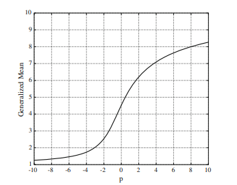
Figure $1[25]$ shows that $\mathscr{H}_{p}{1,2, \ldots, 10}$ varies continuously as $p$ changes from $-10$ to 10 . The arithmetic mean, the geometric mean, and the harmonic mean are special cases of the generalized mean when $p=1, p \rightarrow 0$, and $p=-1$, respectively. Furthermore, the maximum and the minimum values of the numbers can also be approximated from the generalized mean by making $p \rightarrow \infty$ and $p \rightarrow-\infty$, respectively. Note that as $p$ decreases (increases), the generalized mean is more affected by the smaller (larger) numbers than the larger (smaller) ones, i.e., controlling $p$ makes it possible to adjust the contribution of each number to the generalized mean. This characteristic is useful in the situation where data samples should be
differently handled according to their importance, for example, when outliers are contained in the training set.
In [25], it was shown that the generalized mean of a set of positive numbers can be expressed by a nonnegative linear combination of the elements in the set as the following:
$$
\left(\frac{1}{K} \sum_{i=1}^{K} a_{i}^{p}\right)^{1 / p}=c_{1} a_{1}+\cdots+c_{K} a_{K}
$$
Each $c_{i}$ in this equation can be obtained by differentiating this equation with respect to $c_{i}$
$$
c_{i}=\left(\frac{1}{K} \sum_{i=1}^{K} a_{i}^{p}\right)^{\frac{1}{p-1}} \frac{a_{i}^{p-1}}{K}
$$
where $i=1, \ldots, K$. In this chapter, it is further simplified as the following:
$$
\begin{aligned}
\sum_{i=1}^{K} a_{i}^{p} &=b_{1} a_{1}+\cdots+b_{K} a_{K} \
b_{i} &=a_{i}^{p-1}, \quad i=1, \ldots, K
\end{aligned}
$$
Note that each weight $b_{i}$ has the same value of 1 if $p=1$, where the generalized mean becomes the arithmetic mean. It is also noted that, if $p$ is less than one, the weight $b_{i}$ increases as $a_{i}$ decreases. This means that, when $p<1$, the generalized mean is more influenced by the small numbers in $\left{a_{i}\right}_{i=1}^{K}$, and the extent of the influence increases as $p$ decreases. This equation plays an important role in solving the optimization problems using the generalized mean.
统计代写|主成分分析代写Principal Component Analysis代考|Generalized Sample Mean
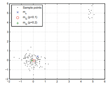
Most conventional PCAs commonly assume that training samples have zero-mean. To satisfy this assumption, all of the samples are subtracted by the sample mean, i.e., $\mathbf{x}{i}-\mathbf{m}{S}$ for $i=1, \ldots, N$, where $\mathbf{m}{S}=\frac{1}{N} \sum{i=1}^{N} \mathbf{x}{i}$. The conventional sample mean can be considered as the center of the samples in the sense of the least square, i.e., $$ \mathbf{m}{S}=\underset{\mathbf{m}}{\arg \min } \frac{1}{N} \sum_{i=1}^{N}\left|\mathbf{x}{i}-\mathbf{m}\right|{2}^{2} .
$$
In (7), a small number of outliers in the training samples dominate the objective function because the objective function in ( 7$)$ is constructed based on the squared distances. To obtain a robust sample mean in the presence of outliers, a new opti-mization problem is formulated by replacing the arithmetic mean in ( 7 ) with the generalized mean as
$$
\mathbf{m}{G}=\underset{\mathbf{m}}{\arg \min }\left(\frac{1}{N} \sum{i=1}^{N}\left(\left|\mathbf{x}{i}-\mathbf{m}\right| |{2}^{2}\right)^{p}\right)^{1 / p}
$$
This problem is equivalent to $(7)$ if $p=1$. As mentioned in the previous subsection, the contribution of a large number to the objective function decreases as $p$ decreases. Thus, the negative effect of outliers can be alleviated if $p<1$. From now on, we will call $\mathbf{m}{G}$ as the generalized sample mean. Using the fact that $x^{p}$ with $p>0$ is a monotonic increasing function of $x$ for $x>0$, this problem can be converted to $$ \mathbf{m}{G}=\underset{\mathbf{m}}{\arg \min } \sum_{i=1}^{N}\left(\left|\mathbf{x}{i}-\mathbf{m}\right|{2}^{2}\right)^{p}
$$
Although the minimization in (8) should be changed into the maximization when $p<0$, we only consider positive values of $p$ in this paper.
The necessary condition for $\mathbf{m}{G}$ to be a local minimum is that the gradient of the objective function in (8) with respect to $\mathrm{m}$ is equal to zero, i.e., $$ \frac{\partial}{\partial \mathbf{m}} \sum{i=1}^{N}\left(\left|\mathbf{x}{i}-\mathbf{m}\right|{2}^{2}\right)^{p}=0
$$
统计代写|主成分分析代写Principal Component Analysis代考|Principal Component Analysis Using Generalized Mean
For a projected sample $\mathbf{W}^{T} \mathbf{x}$, the squared reconstruction error $e(\mathbf{W})$ can be computed as
$$
e(\mathbf{W})=\tilde{\mathbf{x}}^{T} \widetilde{\mathbf{x}}-\tilde{\mathbf{x}}^{T} \mathbf{W} \mathbf{W}^{T} \widetilde{\mathbf{x}}
$$
where $\tilde{\mathbf{x}}=\mathbf{x}-\mathbf{m}$. We use the generalized sample mean $\mathbf{m}{G}$ for $\mathbf{m}$. To prevent outliers corresponding to large $e(\mathbf{W})$ from dominating the objective function, we propose to minimize the following objective function: $$ J{G}(\mathbf{W})=\left(\frac{1}{N} \sum_{i=1}^{N}\left[e_{i}(\mathbf{W})\right]^{p}\right)^{1 / p}
$$
where $e_{i}(\mathbf{W})=\tilde{\mathbf{x}}{i}^{T} \tilde{\mathbf{x}}{i}-\tilde{\mathbf{x}}{i}^{T} \mathbf{W} \mathbf{W}^{T} \tilde{\mathbf{x}}{i}$ is the squared reconstruction error of $\mathbf{x}{i}$ with respect to $\mathbf{W}$. Note that $J{G}(\mathbf{W})$ is formulated by replacing the arithmetic mean in $J_{L_{2}}(\mathbf{W})$ with the generalized mean keeping the use of the Euclidean distance and it is equivalent to $J_{L_{2}}(\mathbf{W})$ if $p=1$. The negative effect raised by outliers is suppressed in the same way as in (8). Also, the solution that minimizes $J_{G}(\mathbf{W})$ is rotational invariant because each $e_{i}(\mathbf{W})$ is measured based on the Euclidean distance. To obtain $\mathbf{W}_{G}$, we develop an iterative optimization method similar to Algorithm $1 .$
主成分分析代考
统计代写|主成分分析代写Principal Component Analysis代考|Generalized Mean
为一个p≠0, 广义均值或幂均值米p的\left{a{i}>0, i=1, \ldots, N\right}\left{a{i}>0, i=1, \ldots, N\right} [20]定义为
\mathcal{M}{p}\left{a{1}, \ldots, a_{N}\right}=\left(\frac{1}{N} \sum_{i=1}^{N} a_ {i}^{p}\right)^{1 / p}\mathcal{M}{p}\left{a{1}, \ldots, a_{N}\right}=\left(\frac{1}{N} \sum_{i=1}^{N} a_ {i}^{p}\right)^{1 / p}
数字1[25]表明Hp1,2,…,10随着不断变化p从变化−10到 10 。算术平均数、几何平均数和调和平均数是广义平均数的特殊情况,当p=1,p→0, 和p=−1, 分别。此外,数字的最大值和最小值也可以通过使p→∞和p→−∞, 分别。请注意,作为p减少(增加),广义均值受较小(较大)数字的影响大于较大(较小)数字,即控制p可以调整每个数字对广义均值的贡献。这个特性在数据样本应该是
根据它们的重要性进行不同的处理,例如,当异常值包含在训练集中时。
在 [25] 中,表明一组正数的广义均值可以通过集合中元素的非负线性组合表示如下:
(1ķ∑一世=1ķ一个一世p)1/p=C1一个1+⋯+Cķ一个ķ
每个C一世在这个方程中,可以通过对这个方程进行微分得到C一世
C一世=(1ķ∑一世=1ķ一个一世p)1p−1一个一世p−1ķ
在哪里一世=1,…,ķ. 在本章中,进一步简化为:
∑一世=1ķ一个一世p=b1一个1+⋯+bķ一个ķ b一世=一个一世p−1,一世=1,…,ķ
注意每个重量b一世具有相同的值 1 如果p=1,其中广义平均值变为算术平均值。还要注意的是,如果p小于一,权重b一世增加为一个一世减少。这意味着,当p<1, 广义均值更受小数的影响\left{a_{i}\right}_{i=1}^{K}\left{a_{i}\right}_{i=1}^{K}, 影响程度随着p减少。该方程在使用广义均值求解优化问题中起着重要作用。
统计代写|主成分分析代写Principal Component Analysis代考|Generalized Sample Mean
大多数传统的 PCA 通常假设训练样本的均值为零。为了满足这个假设,所有样本都减去样本均值,即X一世−米小号为了一世=1,…,ñ, 在哪里米小号=1ñ∑一世=1ñX一世. 传统的样本均值可以认为是最小二乘意义上的样本中心,即
米小号=参数分钟米1ñ∑一世=1ñ|X一世−米|22.
在(7)中,训练样本中的少量异常值支配了目标函数,因为(7)中的目标函数)是根据平方距离构造的。为了在存在异常值的情况下获得稳健的样本均值,通过将 (7) 中的算术均值替换为广义均值来制定一个新的优化问题:
米G=参数分钟米(1ñ∑一世=1ñ(|X一世−米||22)p)1/p
这个问题相当于(7)如果p=1. 如上一小节所述,大数对目标函数的贡献减少为p减少。因此,如果异常值的负面影响可以减轻p<1. 从现在开始,我们将调用米G作为广义样本均值。利用这个事实Xp和p>0是一个单调递增函数X为了X>0,这个问题可以转化为
米G=参数分钟米∑一世=1ñ(|X一世−米|22)p
虽然(8)中的最小化应该变成最大化时p<0,我们只考虑正值p在本文中。
的必要条件米G成为局部最小值是(8)中目标函数的梯度相对于米等于零,即
∂∂米∑一世=1ñ(|X一世−米|22)p=0
统计代写|主成分分析代写Principal Component Analysis代考|Principal Component Analysis Using Generalized Mean
对于投影样本在吨X, 平方重建误差和(在)可以计算为
和(在)=X~吨X~−X~吨在在吨X~
在哪里X~=X−米. 我们使用广义样本均值米G为了米. 防止异常值对应大和(在)为了控制目标函数,我们建议最小化以下目标函数:
ĴG(在)=(1ñ∑一世=1ñ[和一世(在)]p)1/p
在哪里和一世(在)=X~一世吨X~一世−X~一世吨在在吨X~一世是平方重建误差X一世关于在. 注意ĴG(在)是通过替换算术平均值来制定的Ĵ大号2(在)广义均值保持使用欧几里得距离,它等价于Ĵ大号2(在)如果p=1. 异常值引起的负面影响以与(8)相同的方式被抑制。此外,最小化的解决方案ĴG(在)是旋转不变的,因为每个和一世(在)是基于欧几里得距离测量的。获得在G, 我们开发了一种类似于 Algorithm 的迭代优化方法1.

统计代写请认准statistics-lab™. statistics-lab™为您的留学生涯保驾护航。
金融工程代写
金融工程是使用数学技术来解决金融问题。金融工程使用计算机科学、统计学、经济学和应用数学领域的工具和知识来解决当前的金融问题,以及设计新的和创新的金融产品。
非参数统计代写
非参数统计指的是一种统计方法,其中不假设数据来自于由少数参数决定的规定模型;这种模型的例子包括正态分布模型和线性回归模型。
广义线性模型代考
广义线性模型(GLM)归属统计学领域,是一种应用灵活的线性回归模型。该模型允许因变量的偏差分布有除了正态分布之外的其它分布。
术语 广义线性模型(GLM)通常是指给定连续和/或分类预测因素的连续响应变量的常规线性回归模型。它包括多元线性回归,以及方差分析和方差分析(仅含固定效应)。
有限元方法代写
有限元方法(FEM)是一种流行的方法,用于数值解决工程和数学建模中出现的微分方程。典型的问题领域包括结构分析、传热、流体流动、质量运输和电磁势等传统领域。
有限元是一种通用的数值方法,用于解决两个或三个空间变量的偏微分方程(即一些边界值问题)。为了解决一个问题,有限元将一个大系统细分为更小、更简单的部分,称为有限元。这是通过在空间维度上的特定空间离散化来实现的,它是通过构建对象的网格来实现的:用于求解的数值域,它有有限数量的点。边界值问题的有限元方法表述最终导致一个代数方程组。该方法在域上对未知函数进行逼近。[1] 然后将模拟这些有限元的简单方程组合成一个更大的方程系统,以模拟整个问题。然后,有限元通过变化微积分使相关的误差函数最小化来逼近一个解决方案。
tatistics-lab作为专业的留学生服务机构,多年来已为美国、英国、加拿大、澳洲等留学热门地的学生提供专业的学术服务,包括但不限于Essay代写,Assignment代写,Dissertation代写,Report代写,小组作业代写,Proposal代写,Paper代写,Presentation代写,计算机作业代写,论文修改和润色,网课代做,exam代考等等。写作范围涵盖高中,本科,研究生等海外留学全阶段,辐射金融,经济学,会计学,审计学,管理学等全球99%专业科目。写作团队既有专业英语母语作者,也有海外名校硕博留学生,每位写作老师都拥有过硬的语言能力,专业的学科背景和学术写作经验。我们承诺100%原创,100%专业,100%准时,100%满意。
随机分析代写
随机微积分是数学的一个分支,对随机过程进行操作。它允许为随机过程的积分定义一个关于随机过程的一致的积分理论。这个领域是由日本数学家伊藤清在第二次世界大战期间创建并开始的。
时间序列分析代写
随机过程,是依赖于参数的一组随机变量的全体,参数通常是时间。 随机变量是随机现象的数量表现,其时间序列是一组按照时间发生先后顺序进行排列的数据点序列。通常一组时间序列的时间间隔为一恒定值(如1秒,5分钟,12小时,7天,1年),因此时间序列可以作为离散时间数据进行分析处理。研究时间序列数据的意义在于现实中,往往需要研究某个事物其随时间发展变化的规律。这就需要通过研究该事物过去发展的历史记录,以得到其自身发展的规律。
回归分析代写
多元回归分析渐进(Multiple Regression Analysis Asymptotics)属于计量经济学领域,主要是一种数学上的统计分析方法,可以分析复杂情况下各影响因素的数学关系,在自然科学、社会和经济学等多个领域内应用广泛。
MATLAB代写
MATLAB 是一种用于技术计算的高性能语言。它将计算、可视化和编程集成在一个易于使用的环境中,其中问题和解决方案以熟悉的数学符号表示。典型用途包括:数学和计算算法开发建模、仿真和原型制作数据分析、探索和可视化科学和工程图形应用程序开发,包括图形用户界面构建MATLAB 是一个交互式系统,其基本数据元素是一个不需要维度的数组。这使您可以解决许多技术计算问题,尤其是那些具有矩阵和向量公式的问题,而只需用 C 或 Fortran 等标量非交互式语言编写程序所需的时间的一小部分。MATLAB 名称代表矩阵实验室。MATLAB 最初的编写目的是提供对由 LINPACK 和 EISPACK 项目开发的矩阵软件的轻松访问,这两个项目共同代表了矩阵计算软件的最新技术。MATLAB 经过多年的发展,得到了许多用户的投入。在大学环境中,它是数学、工程和科学入门和高级课程的标准教学工具。在工业领域,MATLAB 是高效研究、开发和分析的首选工具。MATLAB 具有一系列称为工具箱的特定于应用程序的解决方案。对于大多数 MATLAB 用户来说非常重要,工具箱允许您学习和应用专业技术。工具箱是 MATLAB 函数(M 文件)的综合集合,可扩展 MATLAB 环境以解决特定类别的问题。可用工具箱的领域包括信号处理、控制系统、神经网络、模糊逻辑、小波、仿真等。