如果你也在 怎样代写回归分析Regression Analysis这个学科遇到相关的难题,请随时右上角联系我们的24/7代写客服。
回归分析是一种强大的统计方法,允许你检查两个或多个感兴趣的变量之间的关系。虽然有许多类型的回归分析,但它们的核心都是考察一个或多个自变量对因变量的影响。
statistics-lab™ 为您的留学生涯保驾护航 在代写回归分析Regression Analysis方面已经树立了自己的口碑, 保证靠谱, 高质且原创的统计Statistics代写服务。我们的专家在代写回归分析Regression Analysis代写方面经验极为丰富,各种代写回归分析Regression Analysis相关的作业也就用不着说。
我们提供的回归分析Regression Analysis及其相关学科的代写,服务范围广, 其中包括但不限于:
- Statistical Inference 统计推断
- Statistical Computing 统计计算
- Advanced Probability Theory 高等楖率论
- Advanced Mathematical Statistics 高等数理统计学
- (Generalized) Linear Models 广义线性模型
- Statistical Machine Learning 统计机器学习
- Longitudinal Data Analysis 纵向数据分析
- Foundations of Data Science 数据科学基础

统计代写|回归分析作业代写Regression Analysis代考|Defining SA
The presence of nonzero correlation results in one $\mathrm{RV}$, $\mathrm{Y}$, in a pair being dependent on the other $\mathrm{RV}$, X. Its global trend depicting a positive relationship is for larger values of $X$ and $Y$ to tend to coincide, for intermediate values of $X$ and $Y$ to tend to coincide, and for smaller values of $X$ and $Y$ to tend to coincide; values of $\mathrm{X}$ are directly proportional to their corresponding values of $Y$. For an indirect (i.e., negative or inverse) relationship, larger values of $X$ tend to coincide with smaller values of $Y$, intermediate values of $X$ and $Y$ tend to coincide, and smaller values of $X$ tend to coincide with larger values of $Y$; values of $X$ are inversely proportional to their corresponding values of $Y$. A random relationship has values of $X$ and $Y$ haphazardly coinciding according to their relative magnitudes.
Autocorrelation transfers this notion of relationships from two RVs to a single RV; the prefix auto means self. Accordingly, $n$ observations have $\mathrm{n}(\mathrm{n}-1)$ possible pairings, one between each observation and the $(n-1)$
remaining observations; each observation always has a correlation of one with itself, and hence these n self-pairings are of little or no interest in terms of correlation. One relevant question asks whether or not an ordering exists that differentiates between two subsets of these $n(n-1)$ pairings such that the ordered subset contains directly correlated observations, whereas the unordered subset contains uncorrelated observations. For data linked to a map, its spatial ordering of attribute values virtually always yields a collection of correlated observations. Because the ordering involved is spatial, the
SA may be defined generically as the arrangement of attribute values on a map for some RV Y such that a map pattern becomes conspicuous by visual inspection. More specifically, positive SA (PSA)-overwhelmingly the most commonly observed type of SA-may be defined as the tendency for similar $Y$ values to cluster on a map. In other words, larger values of $Y$ tend to be surrounded by larger values of $Y$, intermediate values of $Y$ tend to be surrounded by intermediate values of $Y$, and smaller values of $Y$ tend to be surrounded by smaller values of Y. In contrast, NSA-a rarely observed type of SA-may be defined as the tendency for dissimilar $Y$ values to cluster on a map. In other words, larger values of $Y$ tend to be surrounded by smaller values of $Y$, intermediate values of $Y$ tend to be surrounded by intermediate values of $Y$, and smaller values of Y tend to be surrounded by larger values of Y. The absence of $\mathrm{SA}$ indicates a lack of map pattern and a haphazard mixture of attribute values across a map.
统计代写|回归分析作业代写Regression Analysis代考|A mathematical formularization of the first law
The preceding definition of $\mathrm{SA}$ indicates that this concept exists because orderliness, (map) pattern, and systematic concentration, rather than randomness, epitomize real-world geospatial phenomena. Tobler’s $(1969$, P. 7) First Law of Geography captures this notion: “everything is related to everything else, but near things are more related than distant things.” In 2004 the Annals of the American Association of Geographers published commentaries by six prominent geographers (Sui, Barnes, Miller, Phillips, Smith, and Goodchild), together with a reply by Tobler (vol. 94: pp. $269-310$ ) about this notion. Subsequent quantitative SA measurements (e.g., see Section 1.1.3) are mathematical abstractions of this empirical rule.
统计代写|回归分析作业代写Regression Analysis代考|Quantifying spatial relationships
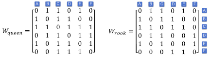
A spatial weights matrix (SWM) is an n-by-n nonnegative (i.e., all of its entries are zero or positive) matrix, say C, describing the geographic relationship structure latent in a georeferenced dataset containing n observations (areal units or point locations in the case of georeferenced data), and has $\mathrm{n}(\mathrm{n}-1) / 2$ potential pairwise, symmetric relationship designations; without invoking symmetry, it has $n(n-1)$ potential relationship designations. Classical statistics assumes that these pairwise relationship designations do not exist (i.e., observation independence). Time-series analyses assume that $(n-1)$ of these pairwise relationship designations are nonzero and asymmetric (dependence is one-directional in time), with perhaps several additional relationship designations to capture seasonality effects. Spatial data mostly assume that between $n-1$ and $3(n-2)$ of these pairwise relationship designations are nonzero and symmetric, with asymmetric relationships usually specified from symmetric ones. The relationship definition rule (often called the neighbor or adjacency rule) is that correlation between attribute values exists for areal unit polygons sharing a common nonzero length boundary (i.e., the rook definition, using a chess move analogy). One extension of this definition is to nonzero length (i.e., point contacts) shared boundaries (i.e., the queen definition, using a chess move analogy). This latter extension tends to increase the number of designated pairwise correlations for administrative polygon surface partitionings by roughly $10 \%$; its asymptotic upper bound is a doubling of pairwise relationships (i.e., the regular square lattice case) for this near-planar situation, which still constitutes a very small percentage of the $n(n-1) / 2$ possible relationshipr. A third extension is to $k>1$ nearest neighbors, which fails to guarantee a connected dual graph structure and for which $\mathrm{k}$ is sufficiently small that it still constitutes a very small percentage of the $n(n-1)$ possible relationships. In all of these specifications of matrix $C$, if areal units $i$ and $j$ are designated polygons/locations with correlated attribute values, then $c_{i j}=1$; otherwise, $c_{i j}=0$. Frequently, matrix $C$ is converted to its often asymmetric row-standardized counterpart, matrix $W$, for which $w_{i j}=c_{i j} / \sum_{j=1}^{n} c_{i j} ; \sum_{j=1}^{n} w_{i j}=1$.
Yet another specification involves inverse distance (i.e., power or negative exponential) between polygon centroids or other points of privilege (e.g., administrative centers, such as capital cities or county seats) within areal unit polygons; these interpoint distances almost always are standardized (i.e., converted to matrix W), perhaps with a carefully chosen power or exponent parameter that essentially equates them to their shared common
boundary topological structure counterpart. Tiefelsdorf, Griffith, and Boots (1999) discuss other schemes defining a SWM that lies between matrices $\mathbf{C}$ and W.
These nearest neighbor and distance-based specifications allow spatial researchers to posit geographic relationship structures for nonpolygon point observations. By generating Thiessen polygon surface partitionings, these researchers also can posit geographic relationships based upon common boundary rules. Eigenvalues of matrices $C$ and $W$, a topic treated in a number of ensuing sections, furnish a quantitative gauge for comparing competing SWMs.
The purpose of a SWM is to define the set of directly correlated observations within a $R V$, enabling the quantification of $S A$ for a georeferenced attribute. It captures the geometric arrangement of attribute values on a map, often in topological terms.
回归分析代写
统计代写|回归分析作业代写Regression Analysis代考|Defining SA
非零相关性的存在导致一个R在, 是, 在一对依赖于另一个R在, X. 其描绘正相关的全局趋势是对于较大的值X和是倾向于重合,对于中间值X和是倾向于重合,并且对于较小的值X和是趋于一致;的值X与它们的相应值成正比是. 对于间接(即负或反向)关系,较大的值X往往与较小的值一致是, 的中间值X和是倾向于重合,并且较小的值X往往与较大的值一致是; 的值X与它们的相应值成反比是. 随机关系的值为X和是根据它们的相对大小随意重合。
自相关将这种关系概念从两个 RV 转移到单个 RV;前缀 auto 表示自我。因此,n观察有n(n−1)可能的配对,在每个观察和(n−1)
剩余的观察;每个观察值总是与自身相关,因此这 n 个自配对在相关性方面几乎没有兴趣或没有兴趣。一个相关的问题是,是否存在区分这两个子集的排序n(n−1)配对使得有序子集包含直接相关的观察,而无序子集包含不相关的观察。对于链接到地图的数据,其属性值的空间排序实际上总是会产生一组相关的观察结果。因为所涉及的排序是空间的,所以
SA 可以一般地定义为一些 RV Y 的地图上的属性值的排列,使得地图图案通过视觉检查变得明显。更具体地说,阳性 SA(PSA)——绝大多数是最常见的 SA 类型——可以定义为相似的趋势是在地图上聚类的值。换句话说,较大的值是往往被较大的值包围是, 的中间值是往往被中间值包围是, 和较小的值是倾向于被较小的 Y 值包围。相比之下,NSA(一种很少观察到的 SA 类型)可以定义为不相似的趋势是在地图上聚类的值。换句话说,较大的值是往往被较小的值包围是, 的中间值是往往被中间值包围是, 较小的 Y 值往往被较大的 Y 值包围。小号一种表示缺乏地图模式和地图上属性值的随意混合。
统计代写|回归分析作业代写Regression Analysis代考|A mathematical formularization of the first law
前面的定义小号一种表明这个概念的存在是因为有序、(地图)模式和系统集中,而不是随机性,是现实世界地理空间现象的缩影。托布勒(1969, P. 7) 地理学第一定律抓住了这个概念:“一切都与其他一切相关,但近处的事物比远处的事物更相关。” 2004 年,美国地理学家协会年鉴发表了六位著名地理学家(Sui、Barnes、Miller、Phillips、Smith 和 Goodchild)的评论,以及 Tobler 的回复(第 94 卷:pp.269−310) 关于这个概念。随后的定量 SA 测量(例如,参见第 1.1.3 节)是该经验规则的数学抽象。
统计代写|回归分析作业代写Regression Analysis代考|Quantifying spatial relationships
空间权重矩阵 (SWM) 是一个 n×n 非负(即其所有条目均为零或正)矩阵,例如 C,描述了包含 n 个观测值(面积单位或点)的地理参考数据集中潜在的地理关系结构在地理参考数据的情况下的位置),并且有n(n−1)/2潜在的成对对称关系名称;在不调用对称的情况下,它有n(n−1)潜在的关系名称。经典统计假设这些成对关系名称不存在(即观察独立性)。时间序列分析假设(n−1)这些成对的关系指定是非零和不对称的(依赖性在时间上是单向的),可能还有几个额外的关系指定来捕捉季节性影响。空间数据大多假设n−1和3(n−2)这些成对关系的指定是非零和对称的,不对称关系通常由对称关系指定。关系定义规则(通常称为邻居或邻接规则)是属性值之间的相关性存在于共享公共非零长度边界的区域单元多边形(即,使用国际象棋移动类比的车定义)。该定义的一个扩展是非零长度(即点接触)共享边界(即,皇后定义,使用国际象棋移动类比)。后一种扩展倾向于将行政多边形表面分区的指定成对相关性的数量大致增加10%; 对于这种接近平面的情况,它的渐近上界是成对关系的两倍(即,正方格子的情况),它仍然占n(n−1)/2可能的关系者。第三个扩展是ķ>1最近的邻居,它不能保证一个连通的对偶图结构,并且ķ足够小,以至于它仍然只占很小的百分比n(n−1)可能的关系。在所有这些规格的矩阵中C, 如果是面积单位一世和j是具有相关属性值的指定多边形/位置,然后C一世j=1; 除此以外,C一世j=0. 通常,矩阵C被转换为其通常不对称的行标准化对应物,矩阵在, 为此在一世j=C一世j/∑j=1nC一世j;∑j=1n在一世j=1.
又一个规范涉及区域单元多边形内多边形质心或其他特权点(例如,行政中心,如首都或县城)之间的反距离(即幂或负指数);这些点间距离几乎总是标准化的(即,转换为矩阵 W),可能使用精心选择的幂或指数参数,基本上将它们等同于它们共享的公共
边界拓扑结构对应物。Tiefelsdorf、Griffith 和 Boots (1999) 讨论了定义位于矩阵之间的 SWM 的其他方案C和W。
这些最近邻和基于距离的规范允许空间研究人员为非多边形点观测设定地理关系结构。通过生成泰森多边形表面分区,这些研究人员还可以根据共同的边界规则确定地理关系。矩阵的特征值C和在,在随后的许多部分中处理的主题,提供了一个定量标准,用于比较竞争的 SWM。
SWM 的目的是定义一组直接相关的观测值R在, 使量化小号一种对于地理参考属性。它通常以拓扑术语捕获地图上属性值的几何排列。

统计代写请认准statistics-lab™. statistics-lab™为您的留学生涯保驾护航。
随机过程代考
在概率论概念中,随机过程是随机变量的集合。 若一随机系统的样本点是随机函数,则称此函数为样本函数,这一随机系统全部样本函数的集合是一个随机过程。 实际应用中,样本函数的一般定义在时间域或者空间域。 随机过程的实例如股票和汇率的波动、语音信号、视频信号、体温的变化,随机运动如布朗运动、随机徘徊等等。
贝叶斯方法代考
贝叶斯统计概念及数据分析表示使用概率陈述回答有关未知参数的研究问题以及统计范式。后验分布包括关于参数的先验分布,和基于观测数据提供关于参数的信息似然模型。根据选择的先验分布和似然模型,后验分布可以解析或近似,例如,马尔科夫链蒙特卡罗 (MCMC) 方法之一。贝叶斯统计概念及数据分析使用后验分布来形成模型参数的各种摘要,包括点估计,如后验平均值、中位数、百分位数和称为可信区间的区间估计。此外,所有关于模型参数的统计检验都可以表示为基于估计后验分布的概率报表。
广义线性模型代考
广义线性模型(GLM)归属统计学领域,是一种应用灵活的线性回归模型。该模型允许因变量的偏差分布有除了正态分布之外的其它分布。
statistics-lab作为专业的留学生服务机构,多年来已为美国、英国、加拿大、澳洲等留学热门地的学生提供专业的学术服务,包括但不限于Essay代写,Assignment代写,Dissertation代写,Report代写,小组作业代写,Proposal代写,Paper代写,Presentation代写,计算机作业代写,论文修改和润色,网课代做,exam代考等等。写作范围涵盖高中,本科,研究生等海外留学全阶段,辐射金融,经济学,会计学,审计学,管理学等全球99%专业科目。写作团队既有专业英语母语作者,也有海外名校硕博留学生,每位写作老师都拥有过硬的语言能力,专业的学科背景和学术写作经验。我们承诺100%原创,100%专业,100%准时,100%满意。
机器学习代写
随着AI的大潮到来,Machine Learning逐渐成为一个新的学习热点。同时与传统CS相比,Machine Learning在其他领域也有着广泛的应用,因此这门学科成为不仅折磨CS专业同学的“小恶魔”,也是折磨生物、化学、统计等其他学科留学生的“大魔王”。学习Machine learning的一大绊脚石在于使用语言众多,跨学科范围广,所以学习起来尤其困难。但是不管你在学习Machine Learning时遇到任何难题,StudyGate专业导师团队都能为你轻松解决。
多元统计分析代考
基础数据: $N$ 个样本, $P$ 个变量数的单样本,组成的横列的数据表
变量定性: 分类和顺序;变量定量:数值
数学公式的角度分为: 因变量与自变量
时间序列分析代写
随机过程,是依赖于参数的一组随机变量的全体,参数通常是时间。 随机变量是随机现象的数量表现,其时间序列是一组按照时间发生先后顺序进行排列的数据点序列。通常一组时间序列的时间间隔为一恒定值(如1秒,5分钟,12小时,7天,1年),因此时间序列可以作为离散时间数据进行分析处理。研究时间序列数据的意义在于现实中,往往需要研究某个事物其随时间发展变化的规律。这就需要通过研究该事物过去发展的历史记录,以得到其自身发展的规律。
回归分析代写
多元回归分析渐进(Multiple Regression Analysis Asymptotics)属于计量经济学领域,主要是一种数学上的统计分析方法,可以分析复杂情况下各影响因素的数学关系,在自然科学、社会和经济学等多个领域内应用广泛。
MATLAB代写
MATLAB 是一种用于技术计算的高性能语言。它将计算、可视化和编程集成在一个易于使用的环境中,其中问题和解决方案以熟悉的数学符号表示。典型用途包括:数学和计算算法开发建模、仿真和原型制作数据分析、探索和可视化科学和工程图形应用程序开发,包括图形用户界面构建MATLAB 是一个交互式系统,其基本数据元素是一个不需要维度的数组。这使您可以解决许多技术计算问题,尤其是那些具有矩阵和向量公式的问题,而只需用 C 或 Fortran 等标量非交互式语言编写程序所需的时间的一小部分。MATLAB 名称代表矩阵实验室。MATLAB 最初的编写目的是提供对由 LINPACK 和 EISPACK 项目开发的矩阵软件的轻松访问,这两个项目共同代表了矩阵计算软件的最新技术。MATLAB 经过多年的发展,得到了许多用户的投入。在大学环境中,它是数学、工程和科学入门和高级课程的标准教学工具。在工业领域,MATLAB 是高效研究、开发和分析的首选工具。MATLAB 具有一系列称为工具箱的特定于应用程序的解决方案。对于大多数 MATLAB 用户来说非常重要,工具箱允许您学习和应用专业技术。工具箱是 MATLAB 函数(M 文件)的综合集合,可扩展 MATLAB 环境以解决特定类别的问题。可用工具箱的领域包括信号处理、控制系统、神经网络、模糊逻辑、小波、仿真等。