如果你也在 怎样代写回归分析Regression Analysis这个学科遇到相关的难题,请随时右上角联系我们的24/7代写客服。
回归分析是一种强大的统计方法,允许你检查两个或多个感兴趣的变量之间的关系。虽然有许多类型的回归分析,但它们的核心都是考察一个或多个自变量对因变量的影响。
statistics-lab™ 为您的留学生涯保驾护航 在代写回归分析Regression Analysis方面已经树立了自己的口碑, 保证靠谱, 高质且原创的统计Statistics代写服务。我们的专家在代写回归分析Regression Analysis代写方面经验极为丰富,各种代写回归分析Regression Analysis相关的作业也就用不着说。
我们提供的回归分析Regression Analysis及其相关学科的代写,服务范围广, 其中包括但不限于:
- Statistical Inference 统计推断
- Statistical Computing 统计计算
- Advanced Probability Theory 高等楖率论
- Advanced Mathematical Statistics 高等数理统计学
- (Generalized) Linear Models 广义线性模型
- Statistical Machine Learning 统计机器学习
- Longitudinal Data Analysis 纵向数据分析
- Foundations of Data Science 数据科学基础
统计代写|回归分析作业代写Regression Analysis代考|An illustrative linear regression example
A pure SA analysis ignores covariates and estimates the SA latent in an attribute variable map pattern. This type of analysis is pertinent to, for example, the construction of histograms for georeferenced RVs or the calculation of Pearson product moment correlation coefficients for pairs of georeferenced RVs, among other things. The MESF linear regression equation, which assumes normally distributed residuals, is the following nonconstant mean-only specification:
$$
\mathbf{Y}=\mathbf{1} \boldsymbol{\beta}{0}+\mathrm{E}{\mathrm{K}} \boldsymbol{\beta}_{\mathrm{E}}+\boldsymbol{\xi} .
$$
One traditional specification error concern here pertains to how closely the response variable Y conforms to a normal distribution. Analysts frequently subject a nonnormal set of attribute values to a $B o x-\operatorname{Cox} /$ Manly transformation to normality (see Griffith, 2013).
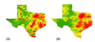
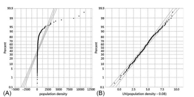
Consider the 2010 population density (PD) across the 254 counties of Texas (see Fig. 3.1A); urban areas are conspicuous in this map pattern, revealing geographic heterogeneity. Raw PD values do not conform closely to a bell-shaped curve (Fig. 3.2A), whereas Box-Cox transformed values LN $(\mathrm{PD}-0.08)$ do (Fig. 3.2B), where LN denotes natural logarithm.
统计代写|回归分析作业代写Regression Analysis代考|The selection of eigenvectors to construct an ESF
The first step in constructing an ESF for the 2010 Texas PD by county is to extract the 254 eigenvectors from the modified SWM $\left(\mathbf{I}-11^{\mathrm{T}} / 254\right) \times$ $\mathbf{C}\left(\mathbf{I}-11^{\mathrm{T}} / 254\right)$, where $0-1$ matrix $\mathrm{C}$ denotes the Texas county SWM, based upon the rook definition of adjacency (see Preface, Fig. P1). Because this PD exhibits PSA, determining an appropriate candidate set of eigenvectors for stepwise regression can begin by setting aside the $149 \mathrm{NSA}$ eigenvectors plus the single eigenvector having a zero eigenvalue (corresponding to the eigenvector proportional to the vector 1 ), which a regression equation already includes for its intercept term. The next step is to determine how many of the 104 PSA eigenvectors to include, counting this number from the largest eigenvalue (i.e., the maximum possible PSA). Chun et al. (2016, p. 75) furnish the following equation to help with this decision:
$$
1+\exp \left{2.1480-\frac{6.1808\left(\mathrm{z}{\mathrm{MC}}+0.6\right)^{0.1742}}{\mathrm{n}{\text {pos }}^{0.1298}}+\frac{3.3534}{\left(\mathrm{z}{\mathrm{MC}}+0.6\right)^{0.1742}}\right} $$ with $\mathrm{n}{\mathrm{Pos}}=104$ (the number of PSA eigenvectors), and $\mathrm{z}{\mathrm{MC}}=13.52$ (the linear regression residuals $z$-score measure of SA) here. This expression indicates that the candidate set should contain the 78 eigenvectors with the largest eigenvalues. Spatial regression analysis using eigenvector spatial filtering One useful criterion for eigenvector selection from the candidate set is the level of significance for each eigenvector’s regression coefficient, which essentially maximizes the linear regression $\mathrm{R}^{2}$ value; other selection criteria could be utilized (see Griffith, 2004). In addition, a stepwise procedure that combines both forward selection and backward elimination supports the construction of a parsimonious ESF. Because the eigenvectors are mutually orthogonal and uncorrelated, the primary factor in eigenvector selection during any given step is the marginal error sum of squares for that step. Of the 78 candidate eigenvectors, 26 were selected using a significance level criterion of $0.10$, accounting for roughly $62.5 \%$ of the variation in logtransformed PD across the counties of Texas (Fig. 3.1B), highlighting the Dallas, Houston, and Austin-San Antonio metropolitan regions and indicating that $\mathrm{SA}$ introduces variance inflation by more than doubling the underlying IID variance. Table $3.1$ summarizes the stepwise selection results, revealing that global (e.g., $\mathbf{E}{2}$ ), regional (e.g., $\mathbf{E}{19}$ ), and local (e.g., $\mathbf{E}{77}$ ) map pattern ${ }^{1}$ components account for the $\mathrm{SA}$ under study and that the Aegree of SA does not determine the selection sequence.
统计代写|回归分析作业代写Regression Analysis代考|Selected criteria for assessing regression models
Once an ESF is constructed, model dingnostics should be performed. The predicted residual error sum of squares (PRESS) statistic is a useful global diagnostic to calculate because it relates to a cross-validation assessment, with the set of covariates being held constant. Values of the ratio PRESS/ESS close to 1, where ESS denotes error sum of squares, indicate good model performance in this context because the corresponding estimated model fitting and prediction error essentially are the same (i.e., the estimated trend line also describes new observations well). Here this values is $376.737 / 355.645=1.059$, implying a very respectable model performance with regard to the cross-validation criterion.
Three features of the linear regression residuals merit assessment. The first concerns normality (Fig. 3.3A); here the Shapiro-Wilk statistic for the linear regrension residuals is $0.98030(p=0.0014)$; the frequency distribution for these residuals differs statistically, but not substantively, from a bell-shaped curve. The second concerns residual SA. The expected value
‘The grouping into global, regional, and local map patterns is subjective. These terms, respectively, refer to $\mathrm{MC} / \mathrm{MC}_{\max }$ (i-e., the maximum $\mathrm{MC}$ ) values in the ranges $0.9-1,0.7-0.9$, and $0.25-0.7$. The maximum MC value here is $1.09798$, which should be used to standardize $\mathrm{MC}$ values to make them comparable across geoggraphic handscapes.
回归分析代写
统计代写|回归分析作业代写Regression Analysis代考|An illustrative linear regression example
纯 SA 分析忽略协变量并估计属性变量映射模式中的潜在 SA。例如,这种类型的分析与地理参考 RV 直方图的构建或地理参考 RV 对的 Pearson 积矩相关系数的计算等有关。假设正态分布残差的 MESF 线性回归方程是以下非常量仅均值规范:
$$
\mathbf{Y}=\mathbf{1} \boldsymbol{\beta} {0}+\mathrm{E} { \mathrm{K}} \boldsymbol{\beta}_{\mathrm{E}}+\boldsymbol{\xi} 。
$$
这里一个传统的规范误差关注点与响应变量 Y 与正态分布的符合程度有关。分析师经常将一组非正态属性值置于乙这X−考克斯/向常态的男子气概转变(参见 Griffith,2013 年)。
考虑 2010 年德克萨斯州 254 个县的人口密度(PD)(见图 3.1A);城市地区在该地图图案中非常显眼,显示出地理异质性。原始 PD 值不符合钟形曲线(图 3.2A),而 Box-Cox 转换值 LN(磷D−0.08)do(图 3.2B),其中 LN 表示自然对数。
统计代写|回归分析作业代写Regression Analysis代考|The selection of eigenvectors to construct an ESF
按县为 2010 年德克萨斯州 PD 构建 ESF 的第一步是从修改后的 SWM 中提取 254 个特征向量(一世−11吨/254)× C(一世−11吨/254), 在哪里0−1矩阵C表示得克萨斯县 SWM,基于邻接的 rook 定义(参见前言,图 P1)。由于此 PD 表现出 PSA,因此可以先将149ñ小号一种特征向量加上具有零特征值的单个特征向量(对应于与向量 1 成比例的特征向量),回归方程已经包括其截距项。下一步是确定要包括多少 104 个 PSA 特征向量,从最大特征值(即最大可能的 PSA)开始计算这个数字。春等人。(2016, p. 75) 提供以下等式来帮助做出这一决定:
1+\exp \left{2.1480-\frac{6.1808\left(\mathrm{z}{\mathrm{MC}}+0.6\right)^{0.1742}}{\mathrm{n}{\text {pos } }^{0.1298}}+\frac{3.3534}{\left(\mathrm{z}{\mathrm{MC}}+0.6\right)^{0.1742}}\right}1+\exp \left{2.1480-\frac{6.1808\left(\mathrm{z}{\mathrm{MC}}+0.6\right)^{0.1742}}{\mathrm{n}{\text {pos } }^{0.1298}}+\frac{3.3534}{\left(\mathrm{z}{\mathrm{MC}}+0.6\right)^{0.1742}}\right}和n磷这s=104(PSA特征向量的数量),和和米C=13.52(线性回归残差和-SA 的得分度量)在这里。这个表达式表明候选集应该包含 78 个特征向量的最大特征值。使用特征向量空间滤波的空间回归分析 从候选集中选择特征向量的一个有用标准是每个特征向量的回归系数的显着性水平,它基本上使线性回归最大化R2价值; 可以使用其他选择标准(参见 Griffith,2004 年)。此外,结合前向选择和后向消除的逐步过程支持简约 ESF 的构建。因为特征向量是相互正交且不相关的,所以在任何给定步骤中选择特征向量的主要因素是该步骤的边际误差平方和。在 78 个候选特征向量中,使用显着性水平标准选择了 26 个0.10, 大致占62.5%得克萨斯州各县的对数转换 PD 的变化(图 3.1B),突出显示达拉斯、休斯顿和奥斯汀-圣安东尼奥大都市区,并表明小号一种通过将基础 IID 方差增加一倍以上来引入方差膨胀。桌子3.1总结了逐步选择的结果,揭示了全局(例如,和2), 地区性的 (例如,和19)和本地(例如,和77) 地图图案1组件占小号一种正在研究中,并且 SA 的 Aegree 不能确定选择顺序。
统计代写|回归分析作业代写Regression Analysis代考|Selected criteria for assessing regression models
构建 ESF 后,应执行模型诊断。预测残差平方和 (PRESS) 统计量是一种有用的全局诊断计算,因为它与交叉验证评估相关,协变量集保持不变。PRESS/ESS 比值接近 1,其中 ESS 表示误差平方和,表明在这种情况下模型性能良好,因为相应的估计模型拟合和预测误差基本相同(即,估计的趋势线也描述了新的观察结果好)。这里的值是376.737/355.645=1.059,这意味着关于交叉验证标准的模型性能非常可观。
线性回归残差的三个特征值得评估。第一个涉及常态(图 3.3A);这里线性回归残差的 Shapiro-Wilk 统计量是0.98030(p=0.0014); 这些残差的频率分布在统计上与钟形曲线不同,但没有实质性差异。第二个涉及剩余 SA。期望值
‘对全球、区域和本地地图模式的分组是主观的。这些术语分别指米C/米C最大限度(即,最大米C) 范围内的值0.9−1,0.7−0.9, 和0.25−0.7. 这里的最大 MC 值为1.09798, 这应该用于标准化米C值以使它们在地理景观中具有可比性。

统计代写请认准statistics-lab™. statistics-lab™为您的留学生涯保驾护航。
随机过程代考
在概率论概念中,随机过程是随机变量的集合。 若一随机系统的样本点是随机函数,则称此函数为样本函数,这一随机系统全部样本函数的集合是一个随机过程。 实际应用中,样本函数的一般定义在时间域或者空间域。 随机过程的实例如股票和汇率的波动、语音信号、视频信号、体温的变化,随机运动如布朗运动、随机徘徊等等。
贝叶斯方法代考
贝叶斯统计概念及数据分析表示使用概率陈述回答有关未知参数的研究问题以及统计范式。后验分布包括关于参数的先验分布,和基于观测数据提供关于参数的信息似然模型。根据选择的先验分布和似然模型,后验分布可以解析或近似,例如,马尔科夫链蒙特卡罗 (MCMC) 方法之一。贝叶斯统计概念及数据分析使用后验分布来形成模型参数的各种摘要,包括点估计,如后验平均值、中位数、百分位数和称为可信区间的区间估计。此外,所有关于模型参数的统计检验都可以表示为基于估计后验分布的概率报表。
广义线性模型代考
广义线性模型(GLM)归属统计学领域,是一种应用灵活的线性回归模型。该模型允许因变量的偏差分布有除了正态分布之外的其它分布。
statistics-lab作为专业的留学生服务机构,多年来已为美国、英国、加拿大、澳洲等留学热门地的学生提供专业的学术服务,包括但不限于Essay代写,Assignment代写,Dissertation代写,Report代写,小组作业代写,Proposal代写,Paper代写,Presentation代写,计算机作业代写,论文修改和润色,网课代做,exam代考等等。写作范围涵盖高中,本科,研究生等海外留学全阶段,辐射金融,经济学,会计学,审计学,管理学等全球99%专业科目。写作团队既有专业英语母语作者,也有海外名校硕博留学生,每位写作老师都拥有过硬的语言能力,专业的学科背景和学术写作经验。我们承诺100%原创,100%专业,100%准时,100%满意。
机器学习代写
随着AI的大潮到来,Machine Learning逐渐成为一个新的学习热点。同时与传统CS相比,Machine Learning在其他领域也有着广泛的应用,因此这门学科成为不仅折磨CS专业同学的“小恶魔”,也是折磨生物、化学、统计等其他学科留学生的“大魔王”。学习Machine learning的一大绊脚石在于使用语言众多,跨学科范围广,所以学习起来尤其困难。但是不管你在学习Machine Learning时遇到任何难题,StudyGate专业导师团队都能为你轻松解决。
多元统计分析代考
基础数据: $N$ 个样本, $P$ 个变量数的单样本,组成的横列的数据表
变量定性: 分类和顺序;变量定量:数值
数学公式的角度分为: 因变量与自变量
时间序列分析代写
随机过程,是依赖于参数的一组随机变量的全体,参数通常是时间。 随机变量是随机现象的数量表现,其时间序列是一组按照时间发生先后顺序进行排列的数据点序列。通常一组时间序列的时间间隔为一恒定值(如1秒,5分钟,12小时,7天,1年),因此时间序列可以作为离散时间数据进行分析处理。研究时间序列数据的意义在于现实中,往往需要研究某个事物其随时间发展变化的规律。这就需要通过研究该事物过去发展的历史记录,以得到其自身发展的规律。
回归分析代写
多元回归分析渐进(Multiple Regression Analysis Asymptotics)属于计量经济学领域,主要是一种数学上的统计分析方法,可以分析复杂情况下各影响因素的数学关系,在自然科学、社会和经济学等多个领域内应用广泛。
MATLAB代写
MATLAB 是一种用于技术计算的高性能语言。它将计算、可视化和编程集成在一个易于使用的环境中,其中问题和解决方案以熟悉的数学符号表示。典型用途包括:数学和计算算法开发建模、仿真和原型制作数据分析、探索和可视化科学和工程图形应用程序开发,包括图形用户界面构建MATLAB 是一个交互式系统,其基本数据元素是一个不需要维度的数组。这使您可以解决许多技术计算问题,尤其是那些具有矩阵和向量公式的问题,而只需用 C 或 Fortran 等标量非交互式语言编写程序所需的时间的一小部分。MATLAB 名称代表矩阵实验室。MATLAB 最初的编写目的是提供对由 LINPACK 和 EISPACK 项目开发的矩阵软件的轻松访问,这两个项目共同代表了矩阵计算软件的最新技术。MATLAB 经过多年的发展,得到了许多用户的投入。在大学环境中,它是数学、工程和科学入门和高级课程的标准教学工具。在工业领域,MATLAB 是高效研究、开发和分析的首选工具。MATLAB 具有一系列称为工具箱的特定于应用程序的解决方案。对于大多数 MATLAB 用户来说非常重要,工具箱允许您学习和应用专业技术。工具箱是 MATLAB 函数(M 文件)的综合集合,可扩展 MATLAB 环境以解决特定类别的问题。可用工具箱的领域包括信号处理、控制系统、神经网络、模糊逻辑、小波、仿真等。