如果你也在 怎样代写实验设计experimental design这个学科遇到相关的难题,请随时右上角联系我们的24/7代写客服。
实验设计是一个概念,用于有效地组织、进行和解释实验结果,确保通过进行少量的试验获得尽可能多的有用信息。
statistics-lab™ 为您的留学生涯保驾护航 在代写实验设计experimental designatistical Modelling方面已经树立了自己的口碑, 保证靠谱, 高质且原创的统计Statistics代写服务。我们的专家在代写实验设计experimental design代写方面经验极为丰富,各种代写实验设计experimental design相关的作业也就用不着说。
我们提供的实验设计experimental design及其相关学科的代写,服务范围广, 其中包括但不限于:
- Statistical Inference 统计推断
- Statistical Computing 统计计算
- Advanced Probability Theory 高等楖率论
- Advanced Mathematical Statistics 高等数理统计学
- (Generalized) Linear Models 广义线性模型
- Statistical Machine Learning 统计机器学习
- Longitudinal Data Analysis 纵向数据分析
- Foundations of Data Science 数据科学基础
统计代写|实验设计作业代写experimental design代考|AGGREGATION OF DATA
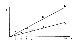
The dummy variable approach of the previous section provides one method of combining together different sets of data. In other situations $1 \mathrm{t}$ may be appropriate to merely sum or average data sets, but it is wise to tread warily for the pattern followed by an individual data set may be quite different from that of the aggregate of the data sets. Aggregation sometimes gives rather disturbing and nonsensical results. Consider Figure $3.9 .1$ in which there is a slight overall downwards trend in the $y$ values as the $x$ values inorease. If there are, as shown, three identifiable subgroups in the data, they may, in fact, suggest a positive trend within each group. In this example, it would be spurious to aggregate the groups. One overall model could be used provided that dummy variables were included to distinguish the $y$-intercepts of each group.
For the lactation records of Appendix $C 3$, it would be useful to fit an overall model to the aggregated data of the five cows. One approach may be to fit a model to each cow’s yield and then to average the estimated coefficients. Problems remain, however, for the model with these averaged coefficients may not fit well any of the individual data sets. Another approach is to average the sets of values of the dependent variable. With different patterns of ylelds, one must ask whether this aggregation is a reasonable thing to do. For example, the maximum yield for cow no, 1 occurred in the sixth week, but for cow no. 5 it occurred in the ninth week. Perhaps the data for each cow should be lagged so that the maxima correspond, and then the appropriate milk yields added (that is $16.30$ of cow no. 1 added to $31.27$ of cow no. 2 etc.). This would ensure that the maxima correspond, but it does not take into account the different shapes of the graphs or that one cow may give milk for a longer time than another. (For convenience, the lactation records here were all truncated to 38 weeks even though some actually gave milk for a longer period).
统计代写|实验设计作业代写experimental design代考|PECULIARITIES OF OBSERVATIONS
In Chapter 3 we considered the relationship between variables $\mathbf{y}$ and $X=\left(x_{1}, x_{2}, \ldots, x_{k}\right)$, that $1 s$, the relationship between the column vectors. In this chapter, we turn our attention to the rows or individual data points
$$
\left(x_{11}, x_{2 i}, \ldots, x_{k i}, y_{1}\right)
$$
We have already seen that the variances of the predicted values and of the residuals depend on the particular values of the predictor variables, $x$. Peculiar values of the $x^{\prime} s$ could be termed sensitive, or high leverage, points as will be explained in Section 2. On the other hand, the observed value of $y$ may be unusual for a given set of $x$ values and y may then be termed an outlier as explained in Section $3 .$
Also, in Sections 6 through 8 , the emphasis is again on the variables in the model and perhaps these topios, more logically, should fall into Chapter 3. They have been added for completeness as they are topics often referred to in other texts.
统计代写|实验设计作业代写experimental design代考|OUTLIERS
Both the prediotor and dependent variables will have their parts to play $1 n$ deciding whether an observation $1 s$ unusual. The predictor variables determine whether a point has hfgh leverage. The value of the dependent variable, $y$, for a given set of $x$ values will determine whether the point is an outlier.
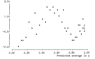
Finst, we consider the residuals, or preferably the studentized residuals. As explained in section 1.3, it is good practice to plot the residuals against the predioted values of $y$ and the predictor variables which are already in the model or which are being considered for inelusion $1 n$ the model. A studentized residual of large absolute value may suggest that an error of measurement or of coding or some such has occurred in the response variable. If the sample size is reasonably large, the observation could be deleted from the analys1s. It is always worthwhile, though, to consider such outliers
very carefully for they may suggest conditions under whioh the model is not valid.
It should be noted that the size of the residuals depends on the model which is fitted. If more, or different, predictor variables are included in the model then it is likely that different points will show up as being potential outliers. It is not possible, then, to completely divorce the detection of outliers from the search for the best model.
Outliers may also be obscured by the presence of points of high leverage for these tend to constrain the prediction curve to pass close to their associated y values. These interrelated effects should warn us to tread cautiously as there is no guaranteed failsafe approach to the problem. Many solutions have been suggested and the interested reader may consult Hoaglin and Welsch (1978). We shall not consider the tests in detail which are contained in this article. To decide whether the i-th observation is an outlier, a fruitful approach is to see the effect that would result from the omission of the 1 -th row of the data. In particular, how would this omission affect the residual at the point and how would it affect the slope of the prediction line?
实验设计代考
统计代写|实验设计作业代写experimental design代考|AGGREGATION OF DATA
上一节的虚拟变量方法提供了一种将不同数据集组合在一起的方法。在其他情况下1吨可能仅适用于汇总或平均数据集,但明智的做法是谨慎行事,因为单个数据集所遵循的模式可能与数据集聚合的模式完全不同。聚合有时会产生相当令人不安和荒谬的结果。考虑图3.9.1其中整体呈小幅下降趋势是的值作为X价值观。如图所示,如果数据中有三个可识别的子组,实际上它们可能表明每个组内都有积极的趋势。在此示例中,聚合组是虚假的。可以使用一个整体模型,前提是包含虚拟变量来区分是的- 每组的截距。
对于附录的泌乳记录C3,将整体模型拟合到五头奶牛的聚合数据中会很有用。一种方法可能是将模型拟合到每头奶牛的产量,然后对估计的系数进行平均。然而,问题仍然存在,因为具有这些平均系数的模型可能无法很好地拟合任何单个数据集。另一种方法是平均因变量的值集。对于不同的 yeld 模式,人们必须问这种聚合是否合理。例如,第 1 号奶牛的最大产量出现在第六周,但第 1 号奶牛的最大产量发生在第 6 周。5 它发生在第九周。也许每头奶牛的数据应该滞后以便最大值对应,然后添加适当的牛奶产量(即16.30牛号 1 添加到31.27牛号 2等)。这将确保最大值对应,但它没有考虑图表的不同形状,或者一头奶牛可能比另一头奶牛产奶的时间更长。(为方便起见,这里的哺乳记录都被截断为 38 周,尽管有些人实际上喂奶的时间更长)。
统计代写|实验设计作业代写experimental design代考|PECULIARITIES OF OBSERVATIONS
在第 3 章中,我们考虑了变量之间的关系是的和X=(X1,X2,…,Xķ), 那1s,列向量之间的关系。在本章中,我们将注意力转向行或单个数据点
(X11,X2一世,…,Xķ一世,是的1)
我们已经看到,预测值和残差的方差取决于预测变量的特定值,X. 独特的价值观X′s可以称为敏感点或高杠杆点,这将在第 2 节中解释。另一方面,观察到的值是的对于给定的一组可能是不寻常的X值和 y 可以称为异常值,如第 1 节所述3.
此外,在第 6 节到第 8 节中,重点再次放在模型中的变量上,从逻辑上讲,这些主题应该属于第 3 章。为了完整起见,添加了它们,因为它们是其他文本中经常提到的主题。
统计代写|实验设计作业代写experimental design代考|OUTLIERS
prediotor 和因变量都将发挥作用1n决定是否观察1s异常。预测变量确定一个点是否具有 hfgh 杠杆。因变量的值,是的, 对于给定的一组X值将确定该点是否为异常值。
Finst,我们考虑残差,或者最好是学生化的残差。如第 1.3 节所述,将残差与是的以及已经在模型中或正在考虑排除的预测变量1n该模型。绝对值较大的学生化残差可能表明响应变量中出现了测量或编码错误等。如果样本量相当大,则可以从分析中删除观察值。不过,考虑这些异常值总是值得的
非常小心,因为他们可能会建议模型无效的条件。
应该注意的是,残差的大小取决于拟合的模型。如果模型中包含更多或不同的预测变量,那么不同的点很可能会显示为潜在的异常值。因此,将异常值的检测与寻找最佳模型完全分开是不可能的。
异常值也可能被高杠杆点的存在所掩盖,因为这些点往往会限制预测曲线接近其相关的 y 值。这些相互关联的影响应该警告我们要谨慎行事,因为没有保证可以解决问题的故障安全方法。已经提出了许多解决方案,感兴趣的读者可以参考 Hoaglin 和 Welsch (1978)。我们将不详细考虑本文中包含的测试。要确定第 i 个观察值是否为异常值,一个富有成效的方法是查看遗漏第 1 行数据所产生的影响。特别是,这种遗漏将如何影响该点的残差以及它将如何影响预测线的斜率?

统计代写请认准statistics-lab™. statistics-lab™为您的留学生涯保驾护航。
金融工程代写
金融工程是使用数学技术来解决金融问题。金融工程使用计算机科学、统计学、经济学和应用数学领域的工具和知识来解决当前的金融问题,以及设计新的和创新的金融产品。
非参数统计代写
非参数统计指的是一种统计方法,其中不假设数据来自于由少数参数决定的规定模型;这种模型的例子包括正态分布模型和线性回归模型。
广义线性模型代考
广义线性模型(GLM)归属统计学领域,是一种应用灵活的线性回归模型。该模型允许因变量的偏差分布有除了正态分布之外的其它分布。
术语 广义线性模型(GLM)通常是指给定连续和/或分类预测因素的连续响应变量的常规线性回归模型。它包括多元线性回归,以及方差分析和方差分析(仅含固定效应)。
有限元方法代写
有限元方法(FEM)是一种流行的方法,用于数值解决工程和数学建模中出现的微分方程。典型的问题领域包括结构分析、传热、流体流动、质量运输和电磁势等传统领域。
有限元是一种通用的数值方法,用于解决两个或三个空间变量的偏微分方程(即一些边界值问题)。为了解决一个问题,有限元将一个大系统细分为更小、更简单的部分,称为有限元。这是通过在空间维度上的特定空间离散化来实现的,它是通过构建对象的网格来实现的:用于求解的数值域,它有有限数量的点。边界值问题的有限元方法表述最终导致一个代数方程组。该方法在域上对未知函数进行逼近。[1] 然后将模拟这些有限元的简单方程组合成一个更大的方程系统,以模拟整个问题。然后,有限元通过变化微积分使相关的误差函数最小化来逼近一个解决方案。
tatistics-lab作为专业的留学生服务机构,多年来已为美国、英国、加拿大、澳洲等留学热门地的学生提供专业的学术服务,包括但不限于Essay代写,Assignment代写,Dissertation代写,Report代写,小组作业代写,Proposal代写,Paper代写,Presentation代写,计算机作业代写,论文修改和润色,网课代做,exam代考等等。写作范围涵盖高中,本科,研究生等海外留学全阶段,辐射金融,经济学,会计学,审计学,管理学等全球99%专业科目。写作团队既有专业英语母语作者,也有海外名校硕博留学生,每位写作老师都拥有过硬的语言能力,专业的学科背景和学术写作经验。我们承诺100%原创,100%专业,100%准时,100%满意。
随机分析代写
随机微积分是数学的一个分支,对随机过程进行操作。它允许为随机过程的积分定义一个关于随机过程的一致的积分理论。这个领域是由日本数学家伊藤清在第二次世界大战期间创建并开始的。
时间序列分析代写
随机过程,是依赖于参数的一组随机变量的全体,参数通常是时间。 随机变量是随机现象的数量表现,其时间序列是一组按照时间发生先后顺序进行排列的数据点序列。通常一组时间序列的时间间隔为一恒定值(如1秒,5分钟,12小时,7天,1年),因此时间序列可以作为离散时间数据进行分析处理。研究时间序列数据的意义在于现实中,往往需要研究某个事物其随时间发展变化的规律。这就需要通过研究该事物过去发展的历史记录,以得到其自身发展的规律。
回归分析代写
多元回归分析渐进(Multiple Regression Analysis Asymptotics)属于计量经济学领域,主要是一种数学上的统计分析方法,可以分析复杂情况下各影响因素的数学关系,在自然科学、社会和经济学等多个领域内应用广泛。
MATLAB代写
MATLAB 是一种用于技术计算的高性能语言。它将计算、可视化和编程集成在一个易于使用的环境中,其中问题和解决方案以熟悉的数学符号表示。典型用途包括:数学和计算算法开发建模、仿真和原型制作数据分析、探索和可视化科学和工程图形应用程序开发,包括图形用户界面构建MATLAB 是一个交互式系统,其基本数据元素是一个不需要维度的数组。这使您可以解决许多技术计算问题,尤其是那些具有矩阵和向量公式的问题,而只需用 C 或 Fortran 等标量非交互式语言编写程序所需的时间的一小部分。MATLAB 名称代表矩阵实验室。MATLAB 最初的编写目的是提供对由 LINPACK 和 EISPACK 项目开发的矩阵软件的轻松访问,这两个项目共同代表了矩阵计算软件的最新技术。MATLAB 经过多年的发展,得到了许多用户的投入。在大学环境中,它是数学、工程和科学入门和高级课程的标准教学工具。在工业领域,MATLAB 是高效研究、开发和分析的首选工具。MATLAB 具有一系列称为工具箱的特定于应用程序的解决方案。对于大多数 MATLAB 用户来说非常重要,工具箱允许您学习和应用专业技术。工具箱是 MATLAB 函数(M 文件)的综合集合,可扩展 MATLAB 环境以解决特定类别的问题。可用工具箱的领域包括信号处理、控制系统、神经网络、模糊逻辑、小波、仿真等。