如果你也在 怎样代写实验设计experimental design这个学科遇到相关的难题,请随时右上角联系我们的24/7代写客服。
实验设计是一个概念,用于有效地组织、进行和解释实验结果,确保通过进行少量的试验获得尽可能多的有用信息。
statistics-lab™ 为您的留学生涯保驾护航 在代写实验设计experimental designatistical Modelling方面已经树立了自己的口碑, 保证靠谱, 高质且原创的统计Statistics代写服务。我们的专家在代写实验设计experimental design代写方面经验极为丰富,各种代写实验设计experimental design相关的作业也就用不着说。
我们提供的实验设计experimental design及其相关学科的代写,服务范围广, 其中包括但不限于:
- Statistical Inference 统计推断
- Statistical Computing 统计计算
- Advanced Probability Theory 高等楖率论
- Advanced Mathematical Statistics 高等数理统计学
- (Generalized) Linear Models 广义线性模型
- Statistical Machine Learning 统计机器学习
- Longitudinal Data Analysis 纵向数据分析
- Foundations of Data Science 数据科学基础
统计代写|实验设计作业代写experimental design代考|Forward Selection
We shall use the heart data of the last two sections to illustrate this. In section 3.5, this data is written in correlation form. If the model is to include only one predictor variable, then $B$ would be chosen as it gives the highest SSR which is also the correlation coefficient with $y$. Before B is placed in the model, we test that it has a significant effect on $y$ by using an $F$-test, or equivalently, a t-test.
We test $\mathrm{H}: B_{2}=0$ in the model $y=B_{0}+B_{2} x_{2}+\varepsilon$
$$
F=(S S R / 1) /(\mathrm{SSE} / 44)=0.657 /(0.342 / 44)=84.7
$$
Clearly, we reject $H$ and include $x_{2}$ in the model. We now try to add
another predictor variable to the model. We look for the variable which, with B, gives the nighest value of SSR. From Table 3.6.1, we see that SSR for $B$ and $C=0.715$ which $1 s$ greater than for $A B=$ $0.667, \mathrm{BD}=0.686, \mathrm{FB}=0.676$, and $\mathrm{BE}=0.659$. Does $\mathrm{C}$ add significantly to SSR over and above B itself? We use the method of reduced models to determine this.
Full model: $y=\beta_{0}+\beta_{2} x_{2}+B_{3} x_{3}+\varepsilon ; \quad$ SSE $=0.285$
Reduced model: $y=\beta_{0}+\beta_{2} x_{2}+\varepsilon ; \quad$ SSE $=0.342$
Difference $=0.05 ?$
$F=0.057 /(0.285 / 43)=8.6$
The tabulated $F$ at $5 \%$ level with 1,43 degrees of freedom = $4.190$ that we reject the reduced model in favor of the full model. We then attempt to add a third variable to the model. The vari= able which adds most to SSR in association with $B$ and $C$ is D as BCD gives an $\mathrm{SSR}=0.718 .$ An $\mathrm{F}$ statistic is evaluated to determine whether $D$ adds significantly to SSR over and above $B$ and $C$.
Ful1 mode1: $y=\beta_{0}+\beta_{2} x_{2}+B_{3} x_{3}+B_{4} x_{4}+\varepsilon ; S S E=0.282$
Reduced model: $y=\beta_{0}+\beta_{2} x_{2}+\beta_{3} x_{3}+E ; \quad$ SSE $=0,285$
Difference $=0.003$
$$
F=0.003 /(0.282 / 42)=0.4
$$
Clearly this is too small to reject the reduced model and we select as the optimal model that with B and $C$ as predictor variables.
统计代写|实验设计作业代写experimental design代考|Backward Elimination
Another approach is to commence with the full model of six prediotor variables and to attempt to remove variables sequentially. In Table 3.6.1, the five predictor model with the greatest SSR Is BCDEF $0.749$ or SSE $=0.251$. To declde if A should be removed, we conpare this SSE with that of the full model using the F statistio.
$$
F=(0.251-0.247) /(0.247 / 39)=0.004 /(0.247 / 39)=0.6
$$
Clearly, the effect of $A$ is not significant and can be removed. We look to remove one of these remaining five variables by considering the SSR for each of the four predictor models. These are:
$\mathrm{BCDE}=0.719, \quad \mathrm{CDEF}=0.703, \quad \mathrm{BDEF}=0.712, \quad \mathrm{FBCD}=0.721$
and $\mathrm{BEFC}=0.741$
We choose this last one with $D$ omitted and test whether this causes a significant reduction in SSR. The full model is now BCDEF and the reduced model is BCEF.
$$
F=0.008 /(0.251 / 40)=1.3
$$
This value is low compared with the $5 \%$ tabulated value for 1 and 40 degrees of freedom which equals $4.08$ so that we proceed to eliminate a further variable. The three variable sums of squares are
$$
C E F=0.684, \quad F B C=0.717, \quad B E F=0.704, \quad E B C=0.717
$$
For either of the models with SSR $=0.717$,
$$
E=0.024 /(0.259 / 41)=3.8
$$
This is slightly below the oritical value of $4.08$ so that we proceed and compare these two models, FBC and $\mathrm{EBC}$, with $\mathrm{BC}$ the last subset of these with two variables.
$$
F=0.002 /(0.283 / 42)=0.3
$$
We are then reduced to the model BC as in the forwand selection process.
There are a number of points to notice about these sequential methods.
统计代写|实验设计作业代写experimental design代考|QUALITATIVE (DUMMY) VARIABLES
It is of ten useful to introduce variables into a model to enable certain specifio effects to be revealed and tested. Usually these take the form of qualitative variables which show up the differences
between subgroups in the data. We shall use an example to explore these ideas.
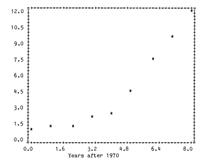
In Example 1.5.1, we listed the value of an Australian stamp (1963 twopenny sepia coloured in the years 1972-1980). We could compare this with the listed value of another stamp, and for few obvious reasons, we have chosen the 1867 New Zealand fourpenny rose colored full face queen. We shall use the same transformation as before, namely
$$
y_{1}=\ln v_{t}, y_{2}=\ln v_{t}
$$
for the Australian and New zealand stamp respectively. The data is given in Table 3.8.1. We could $f$ it a separate model to each stamp, that is, for the Australian stamp
$$
y_{1}=a_{1} 1+\alpha_{2} t_{1}+\varepsilon_{1}
$$
and the New Zealand stamp
$$
\boldsymbol{y}{2}=B{1} \mathbf{1}+B_{2} \mathrm{t}{2}+\varepsilon{2}
$$
If the distributions of the deviations can be assumed to be the same, it will be adrisable to join these models into a single model.
实验设计代考
统计代写|实验设计作业代写experimental design代考|Forward Selection
我们将使用最后两节的心脏数据来说明这一点。在 3.5 节中,该数据以相关形式编写。如果模型只包含一个预测变量,那么乙将被选择,因为它给出了最高的 SSR,这也是与是的. 在将 B 放入模型之前,我们测试它对是的通过使用F-test 或等效的 t 检验。
我们测试H:乙2=0在模型中是的=乙0+乙2X2+e
F=(小号小号R/1)/(小号小号和/44)=0.657/(0.342/44)=84.7
很明显,我们拒绝H并包括X2在模型中。我们现在尝试添加
模型的另一个预测变量。我们寻找与 B 一起给出 SSR 最接近值的变量。从表 3.6.1 中,我们看到 SSR 为乙和C=0.715哪一个1s大于一种乙= 0.667,乙D=0.686,F乙=0.676, 和乙和=0.659. 做C除了 B 本身之外,还显着增加了 SSR?我们使用简化模型的方法来确定这一点。
完整型号:是的=b0+b2X2+乙3X3+e;上证所=0.285
缩小型号:是的=b0+b2X2+e;上证所=0.342
不同之处=0.05?
F=0.057/(0.285/43)=8.6
列表中的F在5%自由度为 1,43 的水平 =4.190我们拒绝简化模型而支持完整模型。然后我们尝试将第三个变量添加到模型中。对 SSR 增加最多的变量乙和C是 D,因为 BCD 给出了小号小号R=0.718.一个F统计数据被评估以确定是否D大大增加了 SSR乙和C.
全模式1:是的=b0+b2X2+乙3X3+乙4X4+e;小号小号和=0.282
缩小型号:是的=b0+b2X2+b3X3+和;上证所=0,285
不同之处=0.003
F=0.003/(0.282/42)=0.4
显然,这太小而无法拒绝简化模型,我们选择 B 和C作为预测变量。
统计代写|实验设计作业代写experimental design代考|Backward Elimination
另一种方法是从六个前因子变量的完整模型开始,并尝试依次删除变量。在表 3.6.1 中,SSR 最大的五个预测模型是 BCDEF0.749或上证所=0.251. 为了确定是否应该删除 A,我们使用 F 统计量将此 SSE 与完整模型的 SSE 进行比较。
F=(0.251−0.247)/(0.247/39)=0.004/(0.247/39)=0.6
很明显,效果一种不重要,可以删除。我们希望通过考虑四个预测模型中的每一个的 SSR 来删除剩余的五个变量之一。这些都是:
乙CD和=0.719,CD和F=0.703,乙D和F=0.712,F乙CD=0.721
和乙和FC=0.741
我们选择最后一个D省略并测试这是否会导致 SSR 显着降低。完整模型现在是 BCDEF,简化模型是 BCEF。
F=0.008/(0.251/40)=1.3
这个值是比较低的5%1 和 40 自由度的列表值,等于4.08以便我们继续消除另一个变量。三个变量平方和是
C和F=0.684,F乙C=0.717,乙和F=0.704,和乙C=0.717
对于带有 SSR 的任一型号=0.717,
和=0.024/(0.259/41)=3.8
略低于原值4.08以便我们继续比较这两个模型,FBC 和和乙C, 和乙C这些的最后一个子集有两个变量。
F=0.002/(0.283/42)=0.3
然后我们被简化为模型 BC,就像在前锋选择过程中一样。
关于这些顺序方法,有许多需要注意的地方。
统计代写|实验设计作业代写experimental design代考|QUALITATIVE (DUMMY) VARIABLES
将变量引入模型以显示和测试某些特定效果是非常有用的。通常这些采用显示差异的定性变量的形式
数据中的子组之间。我们将用一个例子来探索这些想法。
在示例 1.5.1 中,我们列出了澳大利亚邮票的价值(1963 年两便士棕褐色,1972-1980 年)。我们可以将其与另一张邮票的上市价值进行比较,出于几个明显的原因,我们选择了 1867 年新西兰四便士玫瑰色全脸女王。我们将使用与之前相同的变换,即
是的1=ln在吨,是的2=ln在吨
分别为澳大利亚和新西兰邮票。数据见表 3.8.1。我们可以F每个邮票都有一个单独的模型,即澳大利亚邮票
是的1=一种11+一种2吨1+e1
和新西兰邮票
是的2=乙11+乙2吨2+e2
如果可以假设偏差的分布是相同的,那么将这些模型合并为一个模型将是可取的。

统计代写请认准statistics-lab™. statistics-lab™为您的留学生涯保驾护航。
金融工程代写
金融工程是使用数学技术来解决金融问题。金融工程使用计算机科学、统计学、经济学和应用数学领域的工具和知识来解决当前的金融问题,以及设计新的和创新的金融产品。
非参数统计代写
非参数统计指的是一种统计方法,其中不假设数据来自于由少数参数决定的规定模型;这种模型的例子包括正态分布模型和线性回归模型。
广义线性模型代考
广义线性模型(GLM)归属统计学领域,是一种应用灵活的线性回归模型。该模型允许因变量的偏差分布有除了正态分布之外的其它分布。
术语 广义线性模型(GLM)通常是指给定连续和/或分类预测因素的连续响应变量的常规线性回归模型。它包括多元线性回归,以及方差分析和方差分析(仅含固定效应)。
有限元方法代写
有限元方法(FEM)是一种流行的方法,用于数值解决工程和数学建模中出现的微分方程。典型的问题领域包括结构分析、传热、流体流动、质量运输和电磁势等传统领域。
有限元是一种通用的数值方法,用于解决两个或三个空间变量的偏微分方程(即一些边界值问题)。为了解决一个问题,有限元将一个大系统细分为更小、更简单的部分,称为有限元。这是通过在空间维度上的特定空间离散化来实现的,它是通过构建对象的网格来实现的:用于求解的数值域,它有有限数量的点。边界值问题的有限元方法表述最终导致一个代数方程组。该方法在域上对未知函数进行逼近。[1] 然后将模拟这些有限元的简单方程组合成一个更大的方程系统,以模拟整个问题。然后,有限元通过变化微积分使相关的误差函数最小化来逼近一个解决方案。
tatistics-lab作为专业的留学生服务机构,多年来已为美国、英国、加拿大、澳洲等留学热门地的学生提供专业的学术服务,包括但不限于Essay代写,Assignment代写,Dissertation代写,Report代写,小组作业代写,Proposal代写,Paper代写,Presentation代写,计算机作业代写,论文修改和润色,网课代做,exam代考等等。写作范围涵盖高中,本科,研究生等海外留学全阶段,辐射金融,经济学,会计学,审计学,管理学等全球99%专业科目。写作团队既有专业英语母语作者,也有海外名校硕博留学生,每位写作老师都拥有过硬的语言能力,专业的学科背景和学术写作经验。我们承诺100%原创,100%专业,100%准时,100%满意。
随机分析代写
随机微积分是数学的一个分支,对随机过程进行操作。它允许为随机过程的积分定义一个关于随机过程的一致的积分理论。这个领域是由日本数学家伊藤清在第二次世界大战期间创建并开始的。
时间序列分析代写
随机过程,是依赖于参数的一组随机变量的全体,参数通常是时间。 随机变量是随机现象的数量表现,其时间序列是一组按照时间发生先后顺序进行排列的数据点序列。通常一组时间序列的时间间隔为一恒定值(如1秒,5分钟,12小时,7天,1年),因此时间序列可以作为离散时间数据进行分析处理。研究时间序列数据的意义在于现实中,往往需要研究某个事物其随时间发展变化的规律。这就需要通过研究该事物过去发展的历史记录,以得到其自身发展的规律。
回归分析代写
多元回归分析渐进(Multiple Regression Analysis Asymptotics)属于计量经济学领域,主要是一种数学上的统计分析方法,可以分析复杂情况下各影响因素的数学关系,在自然科学、社会和经济学等多个领域内应用广泛。
MATLAB代写
MATLAB 是一种用于技术计算的高性能语言。它将计算、可视化和编程集成在一个易于使用的环境中,其中问题和解决方案以熟悉的数学符号表示。典型用途包括:数学和计算算法开发建模、仿真和原型制作数据分析、探索和可视化科学和工程图形应用程序开发,包括图形用户界面构建MATLAB 是一个交互式系统,其基本数据元素是一个不需要维度的数组。这使您可以解决许多技术计算问题,尤其是那些具有矩阵和向量公式的问题,而只需用 C 或 Fortran 等标量非交互式语言编写程序所需的时间的一小部分。MATLAB 名称代表矩阵实验室。MATLAB 最初的编写目的是提供对由 LINPACK 和 EISPACK 项目开发的矩阵软件的轻松访问,这两个项目共同代表了矩阵计算软件的最新技术。MATLAB 经过多年的发展,得到了许多用户的投入。在大学环境中,它是数学、工程和科学入门和高级课程的标准教学工具。在工业领域,MATLAB 是高效研究、开发和分析的首选工具。MATLAB 具有一系列称为工具箱的特定于应用程序的解决方案。对于大多数 MATLAB 用户来说非常重要,工具箱允许您学习和应用专业技术。工具箱是 MATLAB 函数(M 文件)的综合集合,可扩展 MATLAB 环境以解决特定类别的问题。可用工具箱的领域包括信号处理、控制系统、神经网络、模糊逻辑、小波、仿真等。