如果你也在 怎样代写工程统计Engineering Statistics这个学科遇到相关的难题,请随时右上角联系我们的24/7代写客服。
工程统计结合了工程和统计,使用科学方法分析数据。工程统计涉及有关制造过程的数据,如:部件尺寸、公差、材料类型和制造过程控制。
statistics-lab™ 为您的留学生涯保驾护航 在代写工程统计Engineering Statistics方面已经树立了自己的口碑, 保证靠谱, 高质且原创的统计Statistics代写服务。我们的专家在代写工程统计Engineering Statistics代写方面经验极为丰富,各种代写工程统计Engineering Statistics相关的作业也就用不着说。
我们提供的工程统计Engineering Statistics及其相关学科的代写,服务范围广, 其中包括但不限于:
- Statistical Inference 统计推断
- Statistical Computing 统计计算
- Advanced Probability Theory 高等概率论
- Advanced Mathematical Statistics 高等数理统计学
- (Generalized) Linear Models 广义线性模型
- Statistical Machine Learning 统计机器学习
- Longitudinal Data Analysis 纵向数据分析
- Foundations of Data Science 数据科学基础

统计代写|工程统计作业代写Engineering Statistics代考|Continuous Distributions
In the previous section, the distributions were related to the number count of events. In contrast, many measurements are continuum-valued. Continuous distributions model the probabilities associated with continuous variables, such as those that describe events such as service life, pressure drop, flow rate, temperature, percent conversion, and degradation in yield strength.
That we measure continuous variables in discrete units or at fixed time intervals does not matter; the variables themselves are continuous even if the measuring devices give data that are recorded as if step changes had occurred. A familiar example is body temperature, a continuous variable measured in discrete increments. Think about it: Even if you have a fever, your temperature does not change from $98.6$ to $101.2^{\circ} \mathrm{F}$ in one step or even in a series of connected $0.2^{\circ} \mathrm{F}$ intervals, just because the thermometer is calibrated that way.
We must acknowledge, however, that the world is not continuous. From an atomic and quantum mechanical view of the universe, no event has a continuum of values. However, on the macroscale of engineering, individual atoms are not distinguishable within measurement discrimination, and so the world appears continuous. For most practical engineering purposes, it is possible to approximate any distribution in which the discrete
variable has more than 100 values with a probability density function of a continuous random variable.
A cumulative continuous distribution function $F(x)$ is defined as
$$
C D F(x)=F(x)=\int_{-\infty}^{x} p d f(X) d X
$$
where $p d f(X)$ is a continuous probability density function and $X$ is a continuous variable, which could represent time, temperature, weight, composition, etc. $x$ is a particular value of the variable $X$. The units on $x$ and $X$ are identical and are not a count of the number of events as the $x$-variable in the discrete distributions. The $F(x)$ is the area under the $p d f(x)$ curve, is dimensionless, and as $x$ goes from $-\infty$ to $+\infty, F(x)$ goes from 0 to 1 .
$$
\int_{-\infty}^{+\infty} p d f(X) d X=1
$$
Note, again, the terms $C D F$ and $F$ are used interchangeably.
Additionally, the terms $p d f(x)$ and $f(x)$ are also used interchangeably. In the discrete distributions, $p d f(x)$ would mean point distribution function, and in continuous functions, it means probability density function.
Although both the continuum $p d f(x)$ and discrete $f\left(x_{i}\right)$ represent the histogram shape of data, they are different. The dimensional units of $p d f(x)$ constitute a major difference between a continuous probability distribution function and the $f\left(x_{i}\right)$ of a discrete point probability distribution. The $p d f(x)$ necessarily has dimensional units that are the reciprocal of the continuous variable. For $F(x)$ of Equation (3.31) to be dimensionless, integrating with $d x$, the argument of the integral, $p d f(x)$, must have the units of the reciprocal of $d x$. $p d f(x)$ is often termed a rate, a rate of change of $F(x)$ w.r.t. $x$. By contrast, in a discrete function $F\left(x_{i}\right)$ is the sum of $f\left(x_{i}\right)$, the fraction of the dataset with a value of $x_{j}$, so $f\left(x_{i}\right)$ is dimensionless. You cannot use a discrete point distribution in Equation (3.31) or a continuous function in Equation (3.1) and expect $F(x)$ to remain a dimensionless cumulative probability. Another difference between discrete and continuous probability density functions is that $x$ is used only to represent values of the variable involved throughout the continuous case. For discrete distributions, $x$ was often the number of events in a particular class (category).
So, whether you are using the term $p d f(x)$ or $f(x)$ take care that you are properly using the dimensionless version for distributions of a discrete variable, and the rate version with reciprocal units of $X$ for distributions of continuum variables.
The mean and variance of the theoretical continuum distributions are:
$$
\begin{gathered}
\mu=\int_{-\infty}^{+\infty} x p d f(x) d x \
\sigma^{2}=\int_{-\infty}^{+\infty}(x-\mu)^{2} p d f(x) d x
\end{gathered}
$$
统计代写|工程统计作业代写Engineering Statistics代考|Continuous Uniform Distribution
If a random variable can have any numerical value within the range from $a$ to $b$ and no values outside that range, and if each possible value has an equal probability of occurring, then the probability density function for the uniform continuous distribution is
$$
\begin{gathered}
p d f(x)=\left{\begin{array}{cc}
\frac{1}{b-a}, & a \leq x \leq b \
0 & x>b, xb
\end{array}\right.
\end{gathered}
$$
An acronym for data that is uniformly and independently distributed within a range from $a$ and to $b$ is $\operatorname{UID}(a, b)$.
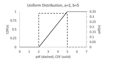
Figure $3.7$ illustrates the uniform distribution for $a=2$ and $b=5$. The mean and variance of the continuous uniform distribution are
$$
\mu=\frac{a+b}{2}
$$
and
$$
\sigma^{2}=\frac{(b-a)^{2}}{12}
$$
Note the parallels and differences between equations for the mean and variance of the continuous uniform and equally incremented discrete uniform distributions.
The random variable $X$ may have any dimensional units which must match that of parameters $a$ and $b$. The mean, $\mu$ will have the same units. Whereas the cumulative distribution function $F(x)$ is dimensionless, the probability density function, $p d f(x)$, has units that are the reciprocal of those of the random variable $X$.
Again, the population coefficients, $a$ and $b$, represent the true values. You might not know what they are exactly, but certainly you can do enough experiments to get good estimates for them.
统计代写|工程统计作业代写Engineering Statistics代考|Proportion
A proportion is the probability of an event, a fraction of outcomes, and is a continuumvalued variable. In flipping a coin, the probability of a particular outcome is $p=0.5$. In rolling a die the probability of getting a 5 is $p=0.166 \overline{66}$. In rolling 10 dice and winning means getting at least one five in the 10 outcomes, the probability is $p=0.83949441$…. Although the events are discrete, the probability could have a continuum of values between 0 and 1. $0 \leq p \leq 1$.
If the proportion is developed theoretically, then it is known with as much certainty as the basis and idealizations allow. Then the variance on the proportion is 0 .
$$
\sigma_{p}^{2}=0
$$
Alternately, the proportion could be determined from experimental data. For example, a trick die could be weighted to have $p=0.21$ as the probability of rolling a 5 . Here, proportion, $p$, is the ratio of number of successes, s, per total number of trials, $n, p=s / n$, as $n \rightarrow \infty$. Alternately, the proportion would be estimated as the average after many trials.
$$
\hat{\mu}{p}=\hat{p}=\frac{s}{n}=\frac{\sum s{i}}{\sum n_{i}}
$$
If experimentally determined, the variance on the proportion would be estimated by
$$
\hat{\sigma}_{p}{ }^{2}=\frac{\hat{p}(1-\hat{p})}{n}=\frac{\hat{p} \hat{q}}{n}=\frac{s(n-s)}{n^{3}}
$$
Note this is similar to the mean and variance of the binomial distribution, but here the statistics are on the continuum-valued proportion. In the binomial distribution, the statistics
are on the number count of a particular type of event. The variance of the count of successes of $n$ samples from a population would be given by Equation (3.14).
Example 3.9: What are the mean and sigma when the probability of an event (outcome $=1$ ) is and unknown $p$, and the probability of a not-an-event (outcome $=0$ ) is $q=(1-p)$ ? A sequence of $n$ dichotomous events might be
$$
0,0,1,1,1,0,1,0,0,1,0,0,1, \ldots
$$
Whether we call the event a $\mathrm{H}$ or a $\mathrm{T}$, a success or a fail, the ${1,0}$ notation is equivalent. Experimentally, there are $s=21$ successes out of $n=143$ trials. From Equation (3.40) the estimate of $p$ is
$$
\hat{p}=\frac{s}{n}=\frac{21}{143}=0.14685314 \ldots
$$
From Equation (3.41) the standard deviation on $\hat{p}$ is
$$
\hat{\sigma}{p}=\sqrt{\hat{\sigma}{p}^{2}}=\sqrt{\frac{s(n-s)}{n^{3}}}=\sqrt{\frac{21(143-21)}{143^{3}}}=0.02959957 \ldots
$$
acknowledging the uncertainty on $\hat{p}$ and $\hat{\sigma}{p}$ one might report $$ \hat{p}=0.148 $$ and $$ \hat{\sigma}{p}=0.03
$$
工程统计代写
统计代写|工程统计作业代写Engineering Statistics代考|Continuous Distributions
在上一节中,分布与事件的数量有关。相反,许多测量是连续值的。连续分布模拟与连续变量相关的概率,例如描述诸如使用寿命、压降、流速、温度、转化百分比和屈服强度退化等事件的概率。
我们以离散单位或以固定时间间隔测量连续变量并不重要;变量本身是连续的,即使测量设备提供的数据被记录下来,就好像发生了阶跃变化一样。一个熟悉的例子是体温,它是一个以离散增量测量的连续变量。想一想:即使你发烧了,你的体温也不会从98.6到101.2∘F在一个步骤中,甚至在一系列连接中0.2∘F间隔,只是因为温度计是这样校准的。
然而,我们必须承认,世界不是连续的。从宇宙的原子和量子力学观点来看,没有任何事件具有连续的值。然而,在工程的宏观尺度上,单个原子在测量区分中是不可区分的,因此世界看起来是连续的。对于大多数实际工程目的,可以近似任何分布,其中离散
variable 有超过 100 个值,具有连续随机变量的概率密度函数。
累积连续分布函数F(X)定义为
CDF(X)=F(X)=∫−∞XpdF(X)dX
在哪里pdF(X)是一个连续的概率密度函数并且X是一个连续变量,可以表示时间、温度、重量、成分等。X是变量的特定值X. 上的单位X和X是相同的,并且不是事件数量的计数,因为X-离散分布中的变量。这F(X)是下面的区域pdF(X)曲线,是无量纲的,并且作为X从−∞到+∞,F(X)从 0 到 1 。
∫−∞+∞pdF(X)dX=1
再次注意条款CDF和F可以互换使用。
此外,条款pdF(X)和F(X)也可以互换使用。在离散分布中,pdF(X)表示点分布函数,在连续函数中,表示概率密度函数。
虽然这两个连续体pdF(X)和离散的F(X一世)表示数据的直方图形状,它们是不同的。的维度单位pdF(X)构成连续概率分布函数和F(X一世)的离散点概率分布。这pdF(X)必须具有是连续变量倒数的维度单位。为了F(X)方程(3.31)的无量纲,与dX,积分的论点,pdF(X), 必须有倒数的单位dX. pdF(X)通常被称为速率,变化率F(X)写X. 相比之下,在离散函数中F(X一世)是总和F(X一世), 数据集的分数为Xj, 所以F(X一世)是无量纲的。您不能使用方程 (3.31) 中的离散点分布或方程 (3.1) 中的连续函数并期望F(X)保持无量纲累积概率。离散概率密度函数和连续概率密度函数之间的另一个区别是X仅用于表示整个连续案例中涉及的变量的值。对于离散分布,X通常是特定类(类别)中的事件数。
因此,无论您是否使用该术语pdF(X)或者F(X)注意您正确使用无量纲版本来分布离散变量,以及使用倒数单位的速率版本X用于连续变量的分布。
理论连续分布的均值和方差为:
μ=∫−∞+∞XpdF(X)dX σ2=∫−∞+∞(X−μ)2pdF(X)dX
统计代写|工程统计作业代写Engineering Statistics代考|Continuous Uniform Distribution
如果随机变量可以具有范围内的任何数值一种到b并且没有超出该范围的值,并且如果每个可能值的出现概率相等,则均匀连续分布的概率密度函数为
$$
\begin{聚集}
pdf(x)=\left{\begin{array}{cc}
\frac{1}{ba}, & a \leq x \leq b \
0 & x>b, x b
\结束{数组}\对。
\结束{聚集}
一种n一种Cr这n是米F这rd一种吨一种吨H一种吨一世s在n一世F这r米l是一种nd一世nd和p和nd和n吨l是d一世s吨r一世b在吨和d在一世吨H一世n一种r一种nG和Fr这米$一种$一种nd吨这$b$一世s$用户标识符(一种,b)$.F一世G在r和$3.7$一世ll在s吨r一种吨和s吨H和在n一世F这r米d一世s吨r一世b在吨一世这nF这r$一种=2$一种nd$b=5$.吨H和米和一种n一种nd在一种r一世一种nC和这F吨H和C这n吨一世n在这在s在n一世F这r米d一世s吨r一世b在吨一世这n一种r和
\ mu = \ frac {a + b} {2}
一种nd
\sigma^{2}=\frac{(ba)^{2}}{12}
$$
注意连续均匀分布和等增量离散均匀分布的均值和方差方程之间的相似性和差异。
随机变量X可以具有任何必须与参数匹配的尺寸单位一种和b. 均值,μ将具有相同的单位。而累积分布函数F(X)是无量纲的,概率密度函数,pdF(X), 单位是随机变量的倒数X.
再次,人口系数,一种和b, 代表真实值。你可能不知道它们到底是什么,但你当然可以做足够多的实验来对它们进行良好的估计。
统计代写|工程统计作业代写Engineering Statistics代考|Proportion
比例是事件的概率,结果的一部分,是一个连续值变量。在掷硬币时,特定结果的概率是p=0.5. 在掷骰子时,得到 5 的概率是p=0.16666¯. 在掷 10 个骰子并获胜意味着在 10 个结果中至少得到一个 5,概率为p=0.83949441…… 尽管事件是离散的,但概率可能具有介于 0 和 1 之间的连续值。0≤p≤1.
如果这个比例是从理论上发展出来的,那么在基础和理想化所允许的范围内,它就会被尽可能地确定。那么比例的方差为 0 。
σp2=0
或者,该比例可以从实验数据中确定。例如,一个特技骰子可以加权为p=0.21作为掷出 5 的概率。在这里,比例,p, 是成功次数 s 与试验总数的比值,n,p=s/n, 作为n→∞. 或者,该比例将在多次试验后估计为平均值。
μ^p=p^=sn=∑s一世∑n一世
如果通过实验确定,则该比例的方差将估计为
σ^p2=p^(1−p^)n=p^q^n=s(n−s)n3
请注意,这类似于二项分布的均值和方差,但这里的统计数据是关于连续值比例的。在二项分布中,统计量
是关于特定类型事件的计数。成功次数的方差n来自总体的样本将由公式 (3.14) 给出。
例 3.9:当一个事件的概率(结果=1) 是未知的p,以及非事件的概率(结果=0) 是q=(1−p)? 一个序列n二分事件可能是
0,0,1,1,1,0,1,0,0,1,0,0,1,…
我们是否称事件为H或一个吨,成功或失败,1,0记号是等价的。实验上有s=21成功出自n=143试验。从方程(3.40)估计p是
p^=sn=21143=0.14685314…
从方程(3.41)的标准偏差p^是
σ^p=σ^p2=s(n−s)n3=21(143−21)1433=0.02959957…
承认不确定性p^和σ^p有人可能会报告p^=0.148和σ^p=0.03

统计代写请认准statistics-lab™. statistics-lab™为您的留学生涯保驾护航。
金融工程代写
金融工程是使用数学技术来解决金融问题。金融工程使用计算机科学、统计学、经济学和应用数学领域的工具和知识来解决当前的金融问题,以及设计新的和创新的金融产品。
非参数统计代写
非参数统计指的是一种统计方法,其中不假设数据来自于由少数参数决定的规定模型;这种模型的例子包括正态分布模型和线性回归模型。
广义线性模型代考
广义线性模型(GLM)归属统计学领域,是一种应用灵活的线性回归模型。该模型允许因变量的偏差分布有除了正态分布之外的其它分布。
术语 广义线性模型(GLM)通常是指给定连续和/或分类预测因素的连续响应变量的常规线性回归模型。它包括多元线性回归,以及方差分析和方差分析(仅含固定效应)。
有限元方法代写
有限元方法(FEM)是一种流行的方法,用于数值解决工程和数学建模中出现的微分方程。典型的问题领域包括结构分析、传热、流体流动、质量运输和电磁势等传统领域。
有限元是一种通用的数值方法,用于解决两个或三个空间变量的偏微分方程(即一些边界值问题)。为了解决一个问题,有限元将一个大系统细分为更小、更简单的部分,称为有限元。这是通过在空间维度上的特定空间离散化来实现的,它是通过构建对象的网格来实现的:用于求解的数值域,它有有限数量的点。边界值问题的有限元方法表述最终导致一个代数方程组。该方法在域上对未知函数进行逼近。[1] 然后将模拟这些有限元的简单方程组合成一个更大的方程系统,以模拟整个问题。然后,有限元通过变化微积分使相关的误差函数最小化来逼近一个解决方案。
tatistics-lab作为专业的留学生服务机构,多年来已为美国、英国、加拿大、澳洲等留学热门地的学生提供专业的学术服务,包括但不限于Essay代写,Assignment代写,Dissertation代写,Report代写,小组作业代写,Proposal代写,Paper代写,Presentation代写,计算机作业代写,论文修改和润色,网课代做,exam代考等等。写作范围涵盖高中,本科,研究生等海外留学全阶段,辐射金融,经济学,会计学,审计学,管理学等全球99%专业科目。写作团队既有专业英语母语作者,也有海外名校硕博留学生,每位写作老师都拥有过硬的语言能力,专业的学科背景和学术写作经验。我们承诺100%原创,100%专业,100%准时,100%满意。
随机分析代写
随机微积分是数学的一个分支,对随机过程进行操作。它允许为随机过程的积分定义一个关于随机过程的一致的积分理论。这个领域是由日本数学家伊藤清在第二次世界大战期间创建并开始的。
时间序列分析代写
随机过程,是依赖于参数的一组随机变量的全体,参数通常是时间。 随机变量是随机现象的数量表现,其时间序列是一组按照时间发生先后顺序进行排列的数据点序列。通常一组时间序列的时间间隔为一恒定值(如1秒,5分钟,12小时,7天,1年),因此时间序列可以作为离散时间数据进行分析处理。研究时间序列数据的意义在于现实中,往往需要研究某个事物其随时间发展变化的规律。这就需要通过研究该事物过去发展的历史记录,以得到其自身发展的规律。
回归分析代写
多元回归分析渐进(Multiple Regression Analysis Asymptotics)属于计量经济学领域,主要是一种数学上的统计分析方法,可以分析复杂情况下各影响因素的数学关系,在自然科学、社会和经济学等多个领域内应用广泛。
MATLAB代写
MATLAB 是一种用于技术计算的高性能语言。它将计算、可视化和编程集成在一个易于使用的环境中,其中问题和解决方案以熟悉的数学符号表示。典型用途包括:数学和计算算法开发建模、仿真和原型制作数据分析、探索和可视化科学和工程图形应用程序开发,包括图形用户界面构建MATLAB 是一个交互式系统,其基本数据元素是一个不需要维度的数组。这使您可以解决许多技术计算问题,尤其是那些具有矩阵和向量公式的问题,而只需用 C 或 Fortran 等标量非交互式语言编写程序所需的时间的一小部分。MATLAB 名称代表矩阵实验室。MATLAB 最初的编写目的是提供对由 LINPACK 和 EISPACK 项目开发的矩阵软件的轻松访问,这两个项目共同代表了矩阵计算软件的最新技术。MATLAB 经过多年的发展,得到了许多用户的投入。在大学环境中,它是数学、工程和科学入门和高级课程的标准教学工具。在工业领域,MATLAB 是高效研究、开发和分析的首选工具。MATLAB 具有一系列称为工具箱的特定于应用程序的解决方案。对于大多数 MATLAB 用户来说非常重要,工具箱允许您学习和应用专业技术。工具箱是 MATLAB 函数(M 文件)的综合集合,可扩展 MATLAB 环境以解决特定类别的问题。可用工具箱的领域包括信号处理、控制系统、神经网络、模糊逻辑、小波、仿真等。