如果你也在 怎样代写应用时间序列分析applied time series analysis这个学科遇到相关的难题,请随时右上角联系我们的24/7代写客服。
时间序列分析applied time series analysis是分析在一个时间间隔内收集的一系列数据点的具体方式。在时间序列分析applied time series analysis中,分析人员在设定的时间段内以一致的时间间隔记录数据点,而不仅仅是间歇性或随机地记录数据点。
statistics-lab™ 为您的留学生涯保驾护航 在代写应用时间序列分析applied time series analysis方面已经树立了自己的口碑, 保证靠谱, 高质且原创的统计Statistics代写服务。我们的专家在代写应用时间序列分析applied time series analysis方面经验极为丰富,各种代写应用时间序列分析applied time series analysis相关的作业也就用不着说。
我们提供的应用时间序列分析applied time series analysis及其相关学科的代写,服务范围广, 其中包括但不限于:
- Statistical Inference 统计推断
- Statistical Computing 统计计算
- Advanced Probability Theory 高等楖率论
- Advanced Mathematical Statistics 高等数理统计学
- (Generalized) Linear Models 广义线性模型
- Statistical Machine Learning 统计机器学习
- Longitudinal Data Analysis 纵向数据分析
- Foundations of Data Science 数据科学基础
统计代写|应用时间序列分析代写applied time series anakysis代考|Likelihood Function of Returns
The partition of Eq. (1.15) can be used to obtain the likelihood function of the log returns $\left{r_{1}, \ldots, r_{T}\right}$ of an asset, where for ease in notation the subscript $i$ is omitted from the log return. If the conditional distribution $f\left(r_{t} \mid r_{t-1}, \ldots, r_{1}, \theta\right)$ is normal with mean $\mu_{t}$ and variance $\sigma_{t}^{2}$, then $\boldsymbol{\theta}$ consists of the parameters in $\mu_{t}$ and $\sigma_{t}^{2}$ and the likelihood function of the data is
$$
f\left(r_{1}, \ldots, r_{T} ; \boldsymbol{\theta}\right)=f\left(r_{1} ; \boldsymbol{\theta}\right) \prod_{t=2}^{T} \frac{1}{\sqrt{2 \pi} \sigma_{t}} \exp \left[\frac{-\left(r_{t}-\mu_{t}\right)^{2}}{2 \sigma_{t}^{2}}\right]
$$
where $f\left(r_{1} ; \theta\right)$ is the marginal density function of the first observation $r_{1}$. The value of $\boldsymbol{\theta}$ that maximizes this likelihood function is the maximum likelihood estimate (MLE) of $\theta$. Since log function is monotone, the MLE can be obtained by maximizing the log likelihood function,
$\ln f\left(r_{1}, \ldots, r_{T} ; \theta\right)=\ln f\left(r_{1} ; \theta\right)-\frac{1}{2} \sum_{t=2}^{T}\left[\ln (2 \pi)+\ln \left(\sigma_{t}^{2}\right)+\frac{\left(r_{t}-\mu_{t}\right)^{2}}{\sigma_{t}^{2}}\right]$
which is casier to handle in practice. Log likelihood function of the data can be obtained in a similar manner if the conditional distribution $f\left(r_{t} \mid r_{t-1}, \ldots, r_{1} ; \theta\right)$ is not normal.
统计代写|应用时间序列分析代写applied time series anakysis代考| Empirical Properties of Returns
The data used in this section are obtained from the Center for Research in Security Prices (CRSP) of the University of Chicago. Dividend payments, if any, are included in the returns. Figure $1.2$ shows the time plots of monthly simple returns and log returns of International Business Machines (IBM) stock from January 1926 to December 1997. A time plot shows the data against the time index. The upper plot is for the simple returns. Figure $1.3$ shows the same plots for the monthly returns of value-weighted market index. As expected, the plots show that the basic patterns of simple and log returns are similar.
Table $1.2$ provides some descriptive statistics of simple and log returns for selected U.S. market indexes and individual stocks. The returns are for daily and monthly sample intervals and are in percentages. The data spans and sample sizes are also given in the table. From the table, we make the following observations. (a) Daily returns of the market indexes and individual stocks tend to have high excess kurtoses. For monthly series, the returns of market indexes have higher excess kurtoses than individual stocks. (b) The mean of a daily return series is close to zero, whereas thatof a monthly return series is slightly larger. (c) Monthly returns have higher standard deviations than daily returns. (d) Among the daily returns, market indexes have smaller standard deviations than individual stocks. This is in agreement with common sense. (e) The skewness is not a serious problem for both daily and monthly
returns. (f) The descriptive statistics show that the difference between simple and log returns is not substantial.
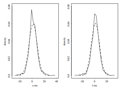
Figure $1.4$ shows the empirical density functions of monthly simple and log returns of IBM stock. Also shown, by a dashed line, in each graph is the normal probability density function evaluated by using the sample mean and standard deviation of IBM returns given in Table 1.2. The plots indicate that the normality assumption is questionable for monthly IBM stock returns. The empirical density function has a higher peak around its mean, but fatter tails than that of the corresponding normal distribution. In other words, the empirical density function is taller, skinnier, but with a wider support than the corresponding normal density.
统计代写|应用时间序列分析代写applied time series anakysis代考|PROCESSES CONSIDERED
Besides the return series, we also consider the volatility process and the behavior of extreme returns of an asset. The volatility process is concerned with the evolution of conditional variance of the return over time. This is a topic of interest because, as shown in Figures $1.2$ and $1.3$, the variabilities of returns vary over time and appear in
clusters. In application, volatility plays an important role in pricing stock options. By extremes of a return series, we mean the large positive or negative returns. Table $1.2$ shows that the minimum and maximum of a return series can be substantial. The negative extreme returns are important in risk management, whereas positive extreme returns are critical to holding a short position. We study properties and applications of extreme returns, such as the frequency of occurrence, the size of an extreme, and the impacts of economic variables on the extremes, in Chapter $7 .$
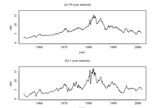
Other financial time series considered in the book include interest rates, exchange rates, bond yields, and quarterly earning per share of a company. Figure $1.5$ shows the time plots of two U.S. monthly interest rates. They are the 10-year and 1-year Treasury constant maturity rates from April 1954 to January 2001. As expected, the two interest rates moved in unison, but the l-year rates appear to be more volatile. Table $1.3$ provides some descriptive statistics for selected U.S. financial time series. The monthly bond returns obtained from CRSP are from January 1942 to December 1999. The interest rates are obtained from the Federal Reserve Bank of St Louis. The weekly 3 -month Treasury Bill rate started on January 8, 1954, and the 6-month rate started on December 12, 1958. Both series ended on February 16, 2001. For the interest rate series, the sample means are proportional to the time to maturity, but the sample standard deviations are inversely proportional to the time to maturity. For
the bond returns, the sample standard deviations are positively related to the time to maturity, whereas the sample means remain stable for all maturities. Most of the series considered have positive excess kurtoses.
With respect to the empirical characteristics of returns shown in Table $1.2$, Chapters 2 to 4 focus on the first four moments of a return series and Chapter 7 on the behavior of minimum and maximum returns. Chapters 8 and 9 are concerned with moments of and the relationships between multiple asset returns, and Chapter 5 addresses properties of asset returns when the time interval is small. An introduction to mathematical finance is given in Chapter 6 .
时间序列分析代写
统计代写|应用时间序列分析代写applied time series anakysis代考|Likelihood Function of Returns
等式的划分。(1.15) 可用于获得对数返回的似然函数\left{r_{1}, \ldots, r_{T}\right}\left{r_{1}, \ldots, r_{T}\right}资产的,为了便于表示,下标一世从日志返回中省略。如果条件分布F(r吨∣r吨−1,…,r1,θ)均值正常μ吨和方差σ吨2, 然后θ由参数组成μ吨和σ吨2数据的似然函数是
F(r1,…,r吨;θ)=F(r1;θ)∏吨=2吨12圆周率σ吨经验[−(r吨−μ吨)22σ吨2]
在哪里F(r1;θ)是第一次观察的边际密度函数r1. 的价值θ使该似然函数最大化的是最大似然估计 (MLE)θ. 由于对数函数是单调的,因此可以通过最大化对数似然函数来获得 MLE,
lnF(r1,…,r吨;θ)=lnF(r1;θ)−12∑吨=2吨[ln(2圆周率)+ln(σ吨2)+(r吨−μ吨)2σ吨2]
这在实践中更容易处理。数据的对数似然函数可以以类似的方式获得,如果条件分布F(r吨∣r吨−1,…,r1;θ)不正常。
统计代写|应用时间序列分析代写applied time series anakysis代考| Empirical Properties of Returns
本节中使用的数据来自芝加哥大学证券价格研究中心 (CRSP)。股息支付(如有)包含在回报中。数字1.2显示了从 1926 年 1 月到 1997 年 12 月国际商业机器公司 (IBM) 股票的每月简单收益和对数收益的时间图。时间图显示了数据与时间指数的关系。上图用于简单回报。数字1.3显示了价值加权市场指数的月收益的相同图。正如预期的那样,这些图显示简单和对数回报的基本模式是相似的。
桌子1.2为选定的美国市场指数和个股提供一些简单和对数回报的描述性统计数据。回报是针对每日和每月的样本间隔,并以百分比表示。表中还给出了数据跨度和样本量。从表中,我们做出以下观察。(a) 市场指数和个股的每日收益往往具有较高的超峰态。对于月度系列,市场指数的回报比个股具有更高的超额峰态。(b) 日收益率序列的平均值接近于零,而月收益率序列的平均值略大。(c) 月回报的标准差高于日回报。(d) 在每日收益中,市场指数的标准差小于个股。这符合常识。
返回。(f) 描述性统计表明简单和对数返回之间的差异不大。
数字1.4显示了 IBM 股票每月简单回报和对数回报的经验密度函数。还用虚线表示,在每张图中,是使用表 1.2 中给出的 IBM 回报的样本均值和标准差评估的正态概率密度函数。这些图表明,对于每月 IBM 股票收益,正态假设是有问题的。经验密度函数在其平均值附近有一个更高的峰值,但比相应的正态分布的尾部更宽。换句话说,经验密度函数更高、更窄,但比相应的正常密度具有更广泛的支持。
统计代写|应用时间序列分析代写applied time series anakysis代考|PROCESSES CONSIDERED
除了收益序列,我们还考虑了波动过程和资产极端收益的行为。波动率过程与收益的条件方差随时间的演变有关。这是一个感兴趣的话题,因为如图所示1.2和1.3,收益的可变性随时间而变化,并出现在
集群。在应用中,波动率对股票期权的定价起着重要作用。通过回报系列的极端,我们指的是大的正回报或负回报。桌子1.2表明回报序列的最小值和最大值可能很大。负极端回报在风险管理中很重要,而正极端回报对于持有空头头寸至关重要。我们研究了极值回报的性质和应用,例如出现频率、极值的大小以及经济变量对极值的影响。7.
书中考虑的其他金融时间序列包括利率、汇率、债券收益率和公司的季度每股收益。数字1.5显示两个美国月利率的时间图。它们是从 1954 年 4 月到 2001 年 1 月的 10 年期和 1 年期国债固定到期利率。正如预期的那样,这两个利率一致移动,但 l 年利率似乎更加波动。桌子1.3为选定的美国金融时间序列提供了一些描述性统计数据。从 CRSP 获得的每月债券收益是从 1942 年 1 月到 1999 年 12 月。利率从圣路易斯联邦储备银行获得。每周 3 个月的国库券利率从 1954 年 1 月 8 日开始,6 个月的利率从 1958 年 12 月 12 日开始。这两个系列都在 2001 年 2 月 16 日结束。对于利率系列,样本均值与到期时间,但样本标准差与到期时间成反比。为了
债券收益率,样本标准差与到期时间正相关,而样本均值在所有到期日都保持稳定。所考虑的大多数系列都具有正的超额峰度。
关于表中回报的经验特征1.2,第 2 章到第 4 章关注回归序列的前四个时刻,第 7 章关注最小和最大收益的行为。第 8 章和第 9 章关注多个资产收益的矩和之间的关系,第 5 章讨论时间间隔较小时资产收益的属性。第 6 章介绍了数学金融。

统计代写请认准statistics-lab™. statistics-lab™为您的留学生涯保驾护航。统计代写|python代写代考
随机过程代考
在概率论概念中,随机过程是随机变量的集合。 若一随机系统的样本点是随机函数,则称此函数为样本函数,这一随机系统全部样本函数的集合是一个随机过程。 实际应用中,样本函数的一般定义在时间域或者空间域。 随机过程的实例如股票和汇率的波动、语音信号、视频信号、体温的变化,随机运动如布朗运动、随机徘徊等等。
贝叶斯方法代考
贝叶斯统计概念及数据分析表示使用概率陈述回答有关未知参数的研究问题以及统计范式。后验分布包括关于参数的先验分布,和基于观测数据提供关于参数的信息似然模型。根据选择的先验分布和似然模型,后验分布可以解析或近似,例如,马尔科夫链蒙特卡罗 (MCMC) 方法之一。贝叶斯统计概念及数据分析使用后验分布来形成模型参数的各种摘要,包括点估计,如后验平均值、中位数、百分位数和称为可信区间的区间估计。此外,所有关于模型参数的统计检验都可以表示为基于估计后验分布的概率报表。
广义线性模型代考
广义线性模型(GLM)归属统计学领域,是一种应用灵活的线性回归模型。该模型允许因变量的偏差分布有除了正态分布之外的其它分布。
statistics-lab作为专业的留学生服务机构,多年来已为美国、英国、加拿大、澳洲等留学热门地的学生提供专业的学术服务,包括但不限于Essay代写,Assignment代写,Dissertation代写,Report代写,小组作业代写,Proposal代写,Paper代写,Presentation代写,计算机作业代写,论文修改和润色,网课代做,exam代考等等。写作范围涵盖高中,本科,研究生等海外留学全阶段,辐射金融,经济学,会计学,审计学,管理学等全球99%专业科目。写作团队既有专业英语母语作者,也有海外名校硕博留学生,每位写作老师都拥有过硬的语言能力,专业的学科背景和学术写作经验。我们承诺100%原创,100%专业,100%准时,100%满意。
机器学习代写
随着AI的大潮到来,Machine Learning逐渐成为一个新的学习热点。同时与传统CS相比,Machine Learning在其他领域也有着广泛的应用,因此这门学科成为不仅折磨CS专业同学的“小恶魔”,也是折磨生物、化学、统计等其他学科留学生的“大魔王”。学习Machine learning的一大绊脚石在于使用语言众多,跨学科范围广,所以学习起来尤其困难。但是不管你在学习Machine Learning时遇到任何难题,StudyGate专业导师团队都能为你轻松解决。
多元统计分析代考
基础数据: $N$ 个样本, $P$ 个变量数的单样本,组成的横列的数据表
变量定性: 分类和顺序;变量定量:数值
数学公式的角度分为: 因变量与自变量
时间序列分析代写
随机过程,是依赖于参数的一组随机变量的全体,参数通常是时间。 随机变量是随机现象的数量表现,其时间序列是一组按照时间发生先后顺序进行排列的数据点序列。通常一组时间序列的时间间隔为一恒定值(如1秒,5分钟,12小时,7天,1年),因此时间序列可以作为离散时间数据进行分析处理。研究时间序列数据的意义在于现实中,往往需要研究某个事物其随时间发展变化的规律。这就需要通过研究该事物过去发展的历史记录,以得到其自身发展的规律。
回归分析代写
多元回归分析渐进(Multiple Regression Analysis Asymptotics)属于计量经济学领域,主要是一种数学上的统计分析方法,可以分析复杂情况下各影响因素的数学关系,在自然科学、社会和经济学等多个领域内应用广泛。
MATLAB代写
MATLAB 是一种用于技术计算的高性能语言。它将计算、可视化和编程集成在一个易于使用的环境中,其中问题和解决方案以熟悉的数学符号表示。典型用途包括:数学和计算算法开发建模、仿真和原型制作数据分析、探索和可视化科学和工程图形应用程序开发,包括图形用户界面构建MATLAB 是一个交互式系统,其基本数据元素是一个不需要维度的数组。这使您可以解决许多技术计算问题,尤其是那些具有矩阵和向量公式的问题,而只需用 C 或 Fortran 等标量非交互式语言编写程序所需的时间的一小部分。MATLAB 名称代表矩阵实验室。MATLAB 最初的编写目的是提供对由 LINPACK 和 EISPACK 项目开发的矩阵软件的轻松访问,这两个项目共同代表了矩阵计算软件的最新技术。MATLAB 经过多年的发展,得到了许多用户的投入。在大学环境中,它是数学、工程和科学入门和高级课程的标准教学工具。在工业领域,MATLAB 是高效研究、开发和分析的首选工具。MATLAB 具有一系列称为工具箱的特定于应用程序的解决方案。对于大多数 MATLAB 用户来说非常重要,工具箱允许您学习和应用专业技术。工具箱是 MATLAB 函数(M 文件)的综合集合,可扩展 MATLAB 环境以解决特定类别的问题。可用工具箱的领域包括信号处理、控制系统、神经网络、模糊逻辑、小波、仿真等。