如果你也在 怎样代写应用随机过程Stochastic process这个学科遇到相关的难题,请随时右上角联系我们的24/7代写客服。
随机过程被定义为随机变量X={Xt:t∈T}的集合,定义在一个共同的概率空间上,时期内的控制和状态轨迹,以使性能指数最小化的过程。
statistics-lab™ 为您的留学生涯保驾护航 在代写应用随机过程Stochastic process方面已经树立了自己的口碑, 保证靠谱, 高质且原创的统计Statistics代写服务。我们的专家在代写应用随机过程Stochastic process代写方面经验极为丰富,各种代写应用随机过程Stochastic process相关的作业也就用不着说。
我们提供的应用随机过程Stochastic process及其相关学科的代写,服务范围广, 其中包括但不限于:
- Statistical Inference 统计推断
- Statistical Computing 统计计算
- Advanced Probability Theory 高等楖率论
- Advanced Mathematical Statistics 高等数理统计学
- (Generalized) Linear Models 广义线性模型
- Statistical Machine Learning 统计机器学习
- Longitudinal Data Analysis 纵向数据分析
- Foundations of Data Science 数据科学基础
统计代写|应用随机过程代写Stochastic process代考|Hypothesis testing
In principle, hypothesis testing problems are straightforward. Consider the case in which we have to decide between two hypotheses with positive probability content, that is, $H_{0}: \theta \in \Theta_{0}$ and $H_{1}: \theta \in \Theta_{1}$. Then, theoretically, the choice of which hypothesis to accept can be treated as a simple decision problem (see Section 2.3). If we accept $H_{0}\left(H_{1}\right)$ when it is true, then we lose nothing. Otherwise, if we accept $H_{0}$, when $H_{1}$ is true, we lose a quantity $l_{01}$ and if we accept $H_{1}$, when $H_{0}$ is true, we lose a quantity $l_{10}$. Then, given the posterior probabilities, $P\left(H_{0} \mid \mathbf{x}\right)$ and $P\left(H_{1} \mid \mathbf{x}\right)$, the expected loss if we accept $H_{0}$ is given by $P\left(H_{1} \mid \mathbf{x}\right) l_{01}$ and the expected loss if we accept $H_{1}$ is $P\left(H_{0} \mid \mathbf{x}\right) l_{10}$. The supported hypothesis is that which minimizes the expected loss. In particular, if $I_{01}=l_{10}$ we should simply select the hypothesis which is most likely a posteriori.
In many cases, such as model selection problems or multiple hypothesis testing problems, the specification of the prior probabilities in favor of each model or hypothesis may be very complicated and an alternative procedure that is not dependent on these prior probabilities may be preferred. The standard tool for such contexts is the Bayes factor.
Definition 2.1: Suppose that $H_{0}$ and $H_{I}$ are two hypotheses with prior probabilities $P\left(H_{0}\right)$ and $P\left(H_{1}\right)$ and posterior probabilities $P\left(H_{0} \mid \mathbf{x}\right)$ and $P\left(H_{1} \mid \mathbf{x}\right)$, respectively. Then, the Bayes factor in favor of $H_{0}$ is
$$
B_{1}^{0}=\frac{P\left(H_{1}\right) P\left(H_{0} \mid \mathbf{x}\right)}{P\left(H_{0}\right) P\left(H_{1} \mid \mathbf{x}\right)}
$$
It is easily shown that the Bayes factor reduces to the marginal likelihood ratio, that is,
$$
B_{1}^{0}=\frac{f\left(\mathbf{x} \mid H_{0}\right)}{f\left(\mathbf{x} \mid H_{1}\right)}
$$
which is independent of the values of $P\left(H_{0}\right)$ and $P\left(H_{1}\right)$ and is, therefore, a measure of the evidence in favor of $H_{0}$ provided by the data. Note, however, that, in general, it is not totally independent of prior information as
$$
f\left(\mathbf{x} \mid H_{0}\right)=\int_{\Theta_{0}} f\left(\mathbf{x} \mid H_{0}, \theta_{0}\right) f\left(\theta_{0} \mid H_{0}\right) d \theta_{0}
$$
which depends on the prior density under $H_{0}$, and similarly for $f\left(\mathbf{x} \mid H_{1}\right)$. Kass and Raftery (1995) presented the following Table 2.1, which indicates the strength of evidence in favor of $H_{0}$ provided by the Bayes factor.
统计代写|应用随机过程代写Stochastic process代考|Prediction
In many applications, rather than being interested in the parameters, we shall be more concerned with the prediction of future observations of the variable of interest. This is especially true in the case of stochastic processes, when we will typically be interested in predicting both the short- and long-term behavior of the process.
For prediction of future values, say $\mathbf{Y}$, of the phenomenon, we use the predictive distribution. To do this, given the current data $\mathbf{x}$, if we knew the value of $\boldsymbol{\theta}$, we would use the conditional predictive distribution $f(\mathbf{y} \mid \mathbf{x}, \boldsymbol{\theta})$. However, since there is uncertainty about $\theta$, modeled through the posterior distribution, $f(\theta \mid \mathbf{x})$, we can integrate this out to calculate the predictive density
$$
f(\mathbf{y} \mid \mathbf{x})=\int f(\mathbf{y} \mid \theta, \mathbf{x}) f(\boldsymbol{\theta} \mid \mathbf{x}) \mathrm{d} \theta
$$
Note that in the case that the sampled values of the phenomenon are conditionally IID, the formula (2.3) simplifies to
$$
f(\mathbf{y} \mid \mathbf{x})=\int f(\mathbf{y} \mid \boldsymbol{\theta}) f(\boldsymbol{\theta} \mid \mathbf{x}) \mathrm{d} \theta
$$
although, in general, to predict the future values of stochastic processes, this simplification will not be available. The predictive density may be used to provide point or set forecasts and test hypotheses about future observations, much as we did earlier.
Example 2.6: In the normal-normal example, to predict the next observation $Y=X_{n+1}$, we have that in the case when a uniform prior was applied, then
$X_{n+1} \mid x \sim \mathrm{N}\left(\bar{x}, \frac{n+1}{n} \sigma^{2}\right)$. Then a predictive $100(1-\alpha) \%$ probability interval is
$$
\left[\bar{x}-z_{\alpha / 2} \sigma \sqrt{(n+1) / n}, \bar{x}+z_{\alpha / 2} \sigma \sqrt{(n+1) / n}\right] \text {. }
$$
统计代写|应用随机过程代写Stochastic process代考|Sensitivity analysis and objective Bayesian methods
As mentioned earlier, prior information may often be elicited from one or more experts. In such cases, the postulated prior distribution will often be an approximation to the expert’s beliefs. In case that different experts disagree, there may be considerable uncertainty about the appropriate prior distribution to apply. In such cases, it is important to assess the sensitivity of any posterior results to changes in the prior distribution. This is typically done by considering appropriate classes of prior distributions, close to the postulated expert prior distribution, and then assessing how the posterior results vary over such classes.
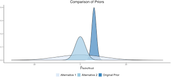
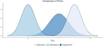
Example 2.8: Assume that the gambler in the gambler’s ruin problem is not certain about her $\operatorname{Be}(5,5)$ prior and wishes to consider the sensitivity of the posterior predictive ruin probability over a reasonable class of alternatives. One possible class of priors that generalizes the gambler’s original prior is
$$
G={f: f \sim \operatorname{Be}(c, c), c>0},
$$
the class of symmetric beta priors. Then, over this class of priors, it can be shown that the gambler’s posterior predictive ruin probability varies between $0.231$, when $c \rightarrow 0$ and $0.8$, when $c \rightarrow \infty$. This shows that there is a large degree of variation of this predictive probability over this class of priors.
When little prior information is available, or in order to promote a more objective analysis, we may try to apply a prior distribution that provides little information and ‘lets the data speak for themselves’. In such cases, we may use a noninformative prior. When $\boldsymbol{\Theta}$ is discrete, a sensible noninformative prior is a uniform distribution. However, when $\boldsymbol{\Theta}$ is continuous, a uniform distribution is not necessarily the best choice. In the univariate case, the most common approach is to use the Jeffreys prior.
Definition 2.3: Suppose that $X \mid \theta \sim f(\cdot \mid \theta)$. The Jeffreys prior for $\theta$ is given by
$$
f(\theta) \propto \sqrt{I(\theta)},
$$
where $I(\theta)=-E_{X}\left[\frac{d^{2}}{d \theta^{2}} \log f(X \mid \theta)\right]$ is the expected Fisher information.
随机过程代写
统计代写|应用随机过程代写Stochastic process代考|Hypothesis testing
原则上,假设检验问题很简单。考虑我们必须在具有正概率内容的两个假设之间做出决定的情况,即H0:θ∈Θ0和H1:θ∈Θ1。然后,理论上,选择接受哪个假设可以被视为一个简单的决策问题(参见第 2.3 节)。如果我们在H0(H1)为真时接受它,那么我们什么都不会丢失。否则,如果我们接受H0,当H1为真时,我们损失一个数量l01,如果我们接受H1,当H0为真时,我们损失一个数量l10. 然后,给定后验概率P(H0∣x)和P(H1∣x),如果我们接受H0由P(H1∣x)l01,如果我们接受H1的预期损失是P(H0∣x)l10。支持的假设是最小化预期损失的假设。特别是,如果I01=l10我们应该简单地选择最有可能是后验的假设。
在许多情况下,例如模型选择问题或多假设检验问题,有利于每个模型或假设的先验概率的规范可能非常复杂,并且可能首选不依赖于这些先验概率的替代程序。这种情况的标准工具是贝叶斯因子。
定义 2.1:假设H0和HI是两个假设,先验概率为P(H0)和P(H1),后验概率为P(H0∣x)和P(H1∣x),分别。那么,有利于H0的贝叶斯因子是
B10=P(H1)P(H0∣x)P(H0)P(H1∣x)
很容易证明贝叶斯因子降低到边际似然比,即
B10=f(x∣H0)f(x∣H1)
它独立于和的值,因此是由数据。但是请注意,一般来说,它并不完全独立于先验信息,因为这取决于先验密度在下,对于也是如此。Kass 和 Raftery (1995) 给出了下表 2.1,表明贝叶斯因子提供的P(H0)P(H1)H0
f(x∣H0)=∫Θ0f(x∣H0,θ0)f(θ0∣H0)dθ0
H0f(x∣H1)H0
统计代写|应用随机过程代写Stochastic process代考|Prediction
在许多应用中,与其对参数感兴趣,不如更关注对感兴趣变量的未来观察结果的预测。在随机过程的情况下尤其如此,当我们通常对预测过程的短期和长期行为感兴趣时。
为了预测未来值,比如Y,我们使用预测分布。为此,给定当前数据x,如果我们知道θ的值,我们将使用条件预测分布f(y∣x,θ)。然而,由于\theta存在不确定性,通过后验分布f(\theta \mid \mathbf{x})θ建模,我们可以将其整合以计算预测密度f(\mathbf{y} \mid \mathbf {x})=\int f(\mathbf{y} \mid \theta, \mathbf{x}) f(\boldsymbol{\theta} \mid \mathbf{x}) \mathrm{d} \thetaf(θ∣x)
f(y∣x)=∫f(y∣θ,x)f(θ∣x)dθ
请注意,在现象的采样值是条件 IID 的情况下,公式 (2.3) 简化为
f(y∣x)=∫f(y∣θ)f(θ∣x)dθ
虽然一般来说,为了预测随机过程的未来值,这种简化将不可用. 预测密度可用于提供点或集合预测并检验关于未来观察的假设,就像我们之前所做的那样。
例 2.6:在正态-正态例子中,为了预测下一个观测Y=Xn+1,我们在应用统一先验的情况下,然后
Xn+1∣x∼N(x¯,n+1nσ2)。那么一个预测的概率区间是100(1−α)%
[x¯−zα/2σ(n+1)/n,x¯+zα/2σ(n+1)/n].
统计代写|应用随机过程代写Stochastic process代考|Sensitivity analysis and objective Bayesian methods
如前所述,通常可以从一位或多位专家那里获得先验信息。在这种情况下,假设的先验分布通常是专家信念的近似值。如果不同的专家不同意,则适用的适当先验分布可能存在相当大的不确定性。在这种情况下,重要的是评估任何后验结果对先验分布变化的敏感性。这通常是通过考虑适当的先验分布类别来完成的,接近假定的专家先验分布,然后评估后验结果如何在这些类别上变化。
例 2.8:假设赌徒破产问题中的赌徒不确定她的先验,并希望考虑后验预测破产概率对合理类别的备选方案的敏感性。概括赌徒原始先验的一类可能的先验是这是一类对称 beta 先验。然后,在这一类先验上,可以证明赌徒的后验预测破产概率在之间变化,当和时,当Be(5,5)
G=f:f∼Be(c,c),c>0,
0.231c→00.8c→∞. 这表明这种预测概率在此类先验上存在很大程度的变化。
当可用的先验信息很少时,或者为了促进更客观的分析,我们可能会尝试应用提供很少信息并“让数据自己说话”的先验分布。在这种情况下,我们可能会使用非信息性先验。当是离散的时,合理的非信息先验是均匀分布。然而,当是连续的时,均匀分布不一定是最佳选择。在单变量情况下,最常见的方法是使用 Jeffreys 先验。定义 2.3:假设。的 Jeffreys 先验由其中ΘΘ
X∣θ∼f(⋅∣θ)θ
f(θ)∝I(θ),
I(θ)=−EX[d2dθ2logf(X∣θ)]是预期的Fisher信息.

统计代写请认准statistics-lab™. statistics-lab™为您的留学生涯保驾护航。
金融工程代写
金融工程是使用数学技术来解决金融问题。金融工程使用计算机科学、统计学、经济学和应用数学领域的工具和知识来解决当前的金融问题,以及设计新的和创新的金融产品。
非参数统计代写
非参数统计指的是一种统计方法,其中不假设数据来自于由少数参数决定的规定模型;这种模型的例子包括正态分布模型和线性回归模型。
广义线性模型代考
广义线性模型(GLM)归属统计学领域,是一种应用灵活的线性回归模型。该模型允许因变量的偏差分布有除了正态分布之外的其它分布。
术语 广义线性模型(GLM)通常是指给定连续和/或分类预测因素的连续响应变量的常规线性回归模型。它包括多元线性回归,以及方差分析和方差分析(仅含固定效应)。
有限元方法代写
有限元方法(FEM)是一种流行的方法,用于数值解决工程和数学建模中出现的微分方程。典型的问题领域包括结构分析、传热、流体流动、质量运输和电磁势等传统领域。
有限元是一种通用的数值方法,用于解决两个或三个空间变量的偏微分方程(即一些边界值问题)。为了解决一个问题,有限元将一个大系统细分为更小、更简单的部分,称为有限元。这是通过在空间维度上的特定空间离散化来实现的,它是通过构建对象的网格来实现的:用于求解的数值域,它有有限数量的点。边界值问题的有限元方法表述最终导致一个代数方程组。该方法在域上对未知函数进行逼近。[1] 然后将模拟这些有限元的简单方程组合成一个更大的方程系统,以模拟整个问题。然后,有限元通过变化微积分使相关的误差函数最小化来逼近一个解决方案。
tatistics-lab作为专业的留学生服务机构,多年来已为美国、英国、加拿大、澳洲等留学热门地的学生提供专业的学术服务,包括但不限于Essay代写,Assignment代写,Dissertation代写,Report代写,小组作业代写,Proposal代写,Paper代写,Presentation代写,计算机作业代写,论文修改和润色,网课代做,exam代考等等。写作范围涵盖高中,本科,研究生等海外留学全阶段,辐射金融,经济学,会计学,审计学,管理学等全球99%专业科目。写作团队既有专业英语母语作者,也有海外名校硕博留学生,每位写作老师都拥有过硬的语言能力,专业的学科背景和学术写作经验。我们承诺100%原创,100%专业,100%准时,100%满意。
随机分析代写
随机微积分是数学的一个分支,对随机过程进行操作。它允许为随机过程的积分定义一个关于随机过程的一致的积分理论。这个领域是由日本数学家伊藤清在第二次世界大战期间创建并开始的。
时间序列分析代写
随机过程,是依赖于参数的一组随机变量的全体,参数通常是时间。 随机变量是随机现象的数量表现,其时间序列是一组按照时间发生先后顺序进行排列的数据点序列。通常一组时间序列的时间间隔为一恒定值(如1秒,5分钟,12小时,7天,1年),因此时间序列可以作为离散时间数据进行分析处理。研究时间序列数据的意义在于现实中,往往需要研究某个事物其随时间发展变化的规律。这就需要通过研究该事物过去发展的历史记录,以得到其自身发展的规律。
回归分析代写
多元回归分析渐进(Multiple Regression Analysis Asymptotics)属于计量经济学领域,主要是一种数学上的统计分析方法,可以分析复杂情况下各影响因素的数学关系,在自然科学、社会和经济学等多个领域内应用广泛。
MATLAB代写
MATLAB 是一种用于技术计算的高性能语言。它将计算、可视化和编程集成在一个易于使用的环境中,其中问题和解决方案以熟悉的数学符号表示。典型用途包括:数学和计算算法开发建模、仿真和原型制作数据分析、探索和可视化科学和工程图形应用程序开发,包括图形用户界面构建MATLAB 是一个交互式系统,其基本数据元素是一个不需要维度的数组。这使您可以解决许多技术计算问题,尤其是那些具有矩阵和向量公式的问题,而只需用 C 或 Fortran 等标量非交互式语言编写程序所需的时间的一小部分。MATLAB 名称代表矩阵实验室。MATLAB 最初的编写目的是提供对由 LINPACK 和 EISPACK 项目开发的矩阵软件的轻松访问,这两个项目共同代表了矩阵计算软件的最新技术。MATLAB 经过多年的发展,得到了许多用户的投入。在大学环境中,它是数学、工程和科学入门和高级课程的标准教学工具。在工业领域,MATLAB 是高效研究、开发和分析的首选工具。MATLAB 具有一系列称为工具箱的特定于应用程序的解决方案。对于大多数 MATLAB 用户来说非常重要,工具箱允许您学习和应用专业技术。工具箱是 MATLAB 函数(M 文件)的综合集合,可扩展 MATLAB 环境以解决特定类别的问题。可用工具箱的领域包括信号处理、控制系统、神经网络、模糊逻辑、小波、仿真等。