如果你也在 怎样代写数值分析和优化numerical analysis and optimazation这个学科遇到相关的难题,请随时右上角联系我们的24/7代写客服。
数值分析是根据数学模型提出的问题,建立求解问题的数值计算方法并进行方法的理论分析,直到编制出算法程序上机计算得到数值结果,以及对结果进行分析。
statistics-lab™ 为您的留学生涯保驾护航 在代写数值分析和优化numerical analysis and optimazation方面已经树立了自己的口碑, 保证靠谱, 高质且原创的统计Statistics代写服务。我们的专家在代写数值分析和优化numerical analysis and optimazation方面经验极为丰富,各种代写数值分析和优化numerical analysis and optimazation相关的作业也就用不着说。
我们提供的数值分析和优化numerical analysis and optimazation及其相关学科的代写,服务范围广, 其中包括但不限于:
- Statistical Inference 统计推断
- Statistical Computing 统计计算
- Advanced Probability Theory 高等楖率论
- Advanced Mathematical Statistics 高等数理统计学
- (Generalized) Linear Models 广义线性模型
- Statistical Machine Learning 统计机器学习
- Longitudinal Data Analysis 纵向数据分析
- Foundations of Data Science 数据科学基础
统计代写|数值分析和优化代写numerical analysis and optimazation代考|Error Testing and Order of Convergence
Often an algorithm first generates an approximation to the solution and then improves this approximation again and again. This is called an iterative numerical process. Often the calculations in each iteration are the same. However, sometimes the calculations are adjusted to reach the solution faster. If the process is successful, the approximate solutions will converge to a solution. Note that it is a solution, not the solution. We will see this beautifully illustrated when considering the fractals generated by Newton’s and Halley’s methods.
More precisely, convergence of a sequence is defined as follows. Let $x_{0}, x_{1}$, $x_{2}, \ldots$ be a sequence (of approximations) and let $x$ be the true solution. We define the absolute error in the $n^{\text {th }}$ iteration as
$$
\epsilon_{\mathrm{n}}=x_{n}-x
$$
The sequence converges to the limit $x$ of the sequence if
$$
\lim {n \rightarrow \infty} \epsilon{n}=0
$$
Note that convergence of a sequence is defined in terms of absolute error.
There are two forms of error testing, one using a target absolute accuracy $\epsilon_{t}$, the other using a target relative error $\delta_{t}$. In the first case the calculation is terminated when
In the second case the calculation is terminated when
Both methods are flawed under certain circumstances. If $x$ is large, say $10^{20}$, and $u=10^{-16}$, then $\epsilon_{n}$ is never likely to be much less than $10^{4}$, so condition $(1.5)$ is unlikely to be satisfied if $\epsilon_{t}$ is chosen too small even when the process converges. On the other hand, if $\left|x_{n}\right|$ is very small, then $\delta_{t}\left|x_{n}\right|$ may underflow and test (1.6) may never be satisfied (unless the error becomes exactly zero). As (1.5) is useful when $(1.6)$ is not, and vice versa, they are combined into a mixed error test. A target error $\eta_{t}$ is prescribed and the calculation is terminated when
$$
\left|\epsilon_{n}\right| \leq \eta_{t}\left(1+\left|x_{n}\right|\right)
$$
If $\left|x_{n}\right|$ is small, $\eta_{t}$ is regarded as target absolute error, or if $\left|x_{n}\right|$ is large $\eta_{t}$ is regarded as target relative error.
Tests such as $(1.7)$ are used in modern numerical software, but we have not addressed the problem of estimating $\epsilon_{n}$, since the true value $x$ is unknown. The simplest formula is
$$
\epsilon_{n} \approx x_{n}-x_{n-1}
$$
However, theoretical research has shown that in a wide class of numerical methods, cases arise where adjacent values in an approximation sequence have the same value, but are both the incorrect answer. Test (1.8) will cause the algorithm to terminate too early with an incorrect solution.
A safer estimate is
$$
\epsilon_{n} \approx\left|x_{n}-x_{n-1}\right|+\left|x_{n-1}-x_{n-2}\right|
$$
but again research has shown that even the approximations of three consecutive iterations can all be the same for certain methods, so (1.9) might not work either. However, in many problems convergence can be tested independently, for example when the inverse of a function can be easily calculated (calculating the $k^{\text {th }}$ power as compared to taking the $k^{\text {th }}$ root). Error and convergence testing should always be fitted to the underlying problem.
统计代写|数值分析和优化代写numerical analysis and optimazation代考|Computational Complexity
A well-designed algorithm should not only be robust, and have a fast rate of convergence, but should also have a reasonable computational complexity. That is, the computation time shall not increase prohibitingly with the size of the problem, because the algorithm is then too slow to be used for large problems.
Suppose that some operation, call it $\odot$, is the most expensive in a particular algorithm. Let $n$ be the size of the problem. If the number of operations of the algorithm can be expressed as $O[f(n)]$ operations of type $\odot$, then we say that the computational complexity is $f(n)$. In other words, we neglect the less expensive operations. However, less expensive operations cannot be neglected, if a large number of them need to be performed for each expensive operation.
For example, in matrix calculations the most expensive operations are multiplications of array elements and array references. Thus in this case the
operation $\odot$ may be defined to be a combination of one multiplication and one or more array references. Let’s consider the multiplication of $n \times n$ matrices $A=\left(A_{i j}\right)$ and $B=\left(B_{i j}\right)$ to form a product $C=\left(C_{i j}\right)$. For each element in $C$, we have to calculate
$$
C_{i j}=\sum_{k=1}^{n} A_{i k} B_{k j}
$$
which requires $n$ multiplications (plus two array references per multiplication). Since there are $n^{2}$ elements in $C$, the computational complexity is $n^{2} \times n=n^{3}$.
Note that processes of lower complexity are absorbed into higher complexity ones and do not change the overall computational complexity of an algorithm. This is the case, unless the processes of lower complexity are performed a large number of times.
For example, if an $n^{2}$ process is performed each time an $n^{3}$ process is performed then, because of
$$
O\left(n^{2}\right)+O\left(n^{3}\right)=O\left(n^{3}\right)
$$
the overall computational complexity is still $n^{3}$. If, however, the $n^{2}$ process was performed $n^{2}$ times each time the $n^{3}$ process was performed, then the computational complexity would be $n^{2} \times n^{2}=n^{4}$.
统计代写|数值分析和优化代写numerical analysis and optimazation代考|Condition
The condition of a problem is inherent to the problem whichever algorithm is used to solve it. The condition number of a numerical problem measures the asymptotically worst case of how much the outcome can change in proportion to small perturbations in the input data. A problem with a low condition number is said to be well-conditioned, while a problem with a high condition number is said to be ill-conditioned. The condition number is a property of the problem and not of the different algorithms that can be used to solve the problem.
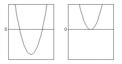
As an example consider the problem where a graph crosses the line $x=0$. Naively one could draw the graph and measure the coordinates of the crossover points. Figure $1.1$ illustrates two cases. In the left-hand problem it would be easier to measure the crossover points, while in the right-hand problem the crossover points lie in a region of candidates. A better (or worse) algorithm would be to use a higher (or lower) resolution. In the chapter on non-linear systems we will encounter many methods to find the roots of a function that is the points where the graph of a function crosses the line $x=0$.
数值分析代写
统计代写|数值分析和优化代写numerical analysis and optimazation代考|Error Testing and Order of Convergence
通常,算法首先会生成解决方案的近似值,然后一次又一次地改进该近似值。这称为迭代数值过程。通常每次迭代中的计算都是相同的。但是,有时会调整计算以更快地得出解决方案。如果该过程成功,则近似解将收敛到一个解。请注意,这是一个解决方案,而不是解决方案。当考虑牛顿和哈雷方法产生的分形时,我们将看到这一点得到了很好的说明。
更准确地说,序列的收敛定义如下。让X0,X1, X2,…是一个(近似值的)序列并让X成为真正的解决方案。我们定义绝对误差nth 迭代为
εn=Xn−X
序列收敛到极限X序列的如果
林n→∞εn=0
请注意,序列的收敛是根据绝对误差定义的。
有两种形式的误差测试,一种使用目标绝对精度ε吨,另一个使用目标相对误差d吨. 在第一种情况下,计算在以下情况下终止。
在第二种情况下,当
两种方法在某些情况下都有缺陷时,计算将终止。如果X很大,说1020, 和在=10−16, 然后εn永远不可能小于104, 所以条件(1.5)不太可能满足,如果ε吨即使过程收敛,也选择得太小。另一方面,如果|Xn|非常小,那么d吨|Xn|可能下溢和测试(1.6)可能永远不会满足(除非误差完全为零)。因为 (1.5) 在以下情况下很有用(1.6)不是,反之亦然,它们组合成一个混合错误测试。目标错误这吨规定和计算终止时
|εn|≤这吨(1+|Xn|)
如果|Xn|是小,这吨被视为目标绝对误差,或者如果|Xn|很大这吨被视为目标相对误差。
测试如(1.7)在现代数值软件中使用,但我们还没有解决估计的问题εn, 因为真实值X是未知的。最简单的公式是
εn≈Xn−Xn−1
然而,理论研究表明,在广泛的数值方法中,会出现近似序列中相邻值具有相同值但都是错误答案的情况。测试 (1.8) 将导致算法过早终止并导致错误的解决方案。
更安全的估计是
εn≈|Xn−Xn−1|+|Xn−1−Xn−2|
但再次研究表明,对于某些方法,即使是三个连续迭代的近似值都可以相同,因此(1.9)也可能不起作用。然而,在许多问题中,收敛性可以独立测试,例如当函数的逆函数可以很容易地计算时(计算ķth 与采取权力相比ķth 根)。误差和收敛性测试应始终适用于潜在问题。
统计代写|数值分析和优化代写numerical analysis and optimazation代考|Computational Complexity
一个设计良好的算法不仅应该是健壮的,并且具有快速的收敛速度,还应该具有合理的计算复杂度。也就是说,计算时间不会随着问题的大小而增加,因为算法太慢而不能用于大问题。
假设一些操作,调用它⊙, 是特定算法中最昂贵的。让n是问题的大小。如果算法的运算次数可以表示为这[F(n)]类型的操作⊙,那么我们说计算复杂度是F(n). 换句话说,我们忽略了成本较低的操作。但是,如果需要为每个昂贵的操作执行大量操作,则不能忽略成本较低的操作。
例如,在矩阵计算中,最昂贵的操作是数组元素和数组引用的乘法。因此在这种情况下
手术⊙可以定义为一个乘法和一个或多个数组引用的组合。让我们考虑乘法n×n矩阵一种=(一种一世j)和乙=(乙一世j)形成一个产品C=(C一世j). 对于每个元素C,我们必须计算
C一世j=∑ķ=1n一种一世ķ乙ķj
这需要n乘法(每次乘法加上两个数组引用)。既然有n2中的元素C,计算复杂度为n2×n=n3.
请注意,较低复杂度的过程被吸收到较高复杂度的过程中,并且不会改变算法的整体计算复杂度。情况就是这样,除非低复杂度的过程被执行很多次。
例如,如果一个n2每次执行一个过程n3然后执行该过程,因为
这(n2)+这(n3)=这(n3)
整体计算复杂度仍然n3. 然而,如果n2进行了处理n2每次n3执行过程,那么计算复杂度将是n2×n2=n4.
统计代写|数值分析和优化代写numerical analysis and optimazation代考|Condition
无论使用哪种算法解决问题,问题的条件都是问题所固有的。数值问题的条件数衡量的是结果与输入数据中的小扰动成比例的变化程度的渐近最坏情况。条件数低的问题被称为条件良好的问题,而条件数高的问题被称为病态问题。条件数是问题的属性,而不是可用于解决问题的不同算法的属性。
作为一个例子,考虑一个图形越界的问题X=0. 可以天真地绘制图形并测量交叉点的坐标。数字1.1说明了两种情况。在左手问题中,测量交叉点会更容易,而在右手问题中,交叉点位于候选区域中。更好(或更差)的算法是使用更高(或更低)的分辨率。在关于非线性系统的章节中,我们将遇到许多方法来找到函数的根,即函数的图形与直线相交的点X=0.

统计代写请认准statistics-lab™. statistics-lab™为您的留学生涯保驾护航。统计代写|python代写代考
随机过程代考
在概率论概念中,随机过程是随机变量的集合。 若一随机系统的样本点是随机函数,则称此函数为样本函数,这一随机系统全部样本函数的集合是一个随机过程。 实际应用中,样本函数的一般定义在时间域或者空间域。 随机过程的实例如股票和汇率的波动、语音信号、视频信号、体温的变化,随机运动如布朗运动、随机徘徊等等。
贝叶斯方法代考
贝叶斯统计概念及数据分析表示使用概率陈述回答有关未知参数的研究问题以及统计范式。后验分布包括关于参数的先验分布,和基于观测数据提供关于参数的信息似然模型。根据选择的先验分布和似然模型,后验分布可以解析或近似,例如,马尔科夫链蒙特卡罗 (MCMC) 方法之一。贝叶斯统计概念及数据分析使用后验分布来形成模型参数的各种摘要,包括点估计,如后验平均值、中位数、百分位数和称为可信区间的区间估计。此外,所有关于模型参数的统计检验都可以表示为基于估计后验分布的概率报表。
广义线性模型代考
广义线性模型(GLM)归属统计学领域,是一种应用灵活的线性回归模型。该模型允许因变量的偏差分布有除了正态分布之外的其它分布。
statistics-lab作为专业的留学生服务机构,多年来已为美国、英国、加拿大、澳洲等留学热门地的学生提供专业的学术服务,包括但不限于Essay代写,Assignment代写,Dissertation代写,Report代写,小组作业代写,Proposal代写,Paper代写,Presentation代写,计算机作业代写,论文修改和润色,网课代做,exam代考等等。写作范围涵盖高中,本科,研究生等海外留学全阶段,辐射金融,经济学,会计学,审计学,管理学等全球99%专业科目。写作团队既有专业英语母语作者,也有海外名校硕博留学生,每位写作老师都拥有过硬的语言能力,专业的学科背景和学术写作经验。我们承诺100%原创,100%专业,100%准时,100%满意。
机器学习代写
随着AI的大潮到来,Machine Learning逐渐成为一个新的学习热点。同时与传统CS相比,Machine Learning在其他领域也有着广泛的应用,因此这门学科成为不仅折磨CS专业同学的“小恶魔”,也是折磨生物、化学、统计等其他学科留学生的“大魔王”。学习Machine learning的一大绊脚石在于使用语言众多,跨学科范围广,所以学习起来尤其困难。但是不管你在学习Machine Learning时遇到任何难题,StudyGate专业导师团队都能为你轻松解决。
多元统计分析代考
基础数据: $N$ 个样本, $P$ 个变量数的单样本,组成的横列的数据表
变量定性: 分类和顺序;变量定量:数值
数学公式的角度分为: 因变量与自变量
时间序列分析代写
随机过程,是依赖于参数的一组随机变量的全体,参数通常是时间。 随机变量是随机现象的数量表现,其时间序列是一组按照时间发生先后顺序进行排列的数据点序列。通常一组时间序列的时间间隔为一恒定值(如1秒,5分钟,12小时,7天,1年),因此时间序列可以作为离散时间数据进行分析处理。研究时间序列数据的意义在于现实中,往往需要研究某个事物其随时间发展变化的规律。这就需要通过研究该事物过去发展的历史记录,以得到其自身发展的规律。
回归分析代写
多元回归分析渐进(Multiple Regression Analysis Asymptotics)属于计量经济学领域,主要是一种数学上的统计分析方法,可以分析复杂情况下各影响因素的数学关系,在自然科学、社会和经济学等多个领域内应用广泛。
MATLAB代写
MATLAB 是一种用于技术计算的高性能语言。它将计算、可视化和编程集成在一个易于使用的环境中,其中问题和解决方案以熟悉的数学符号表示。典型用途包括:数学和计算算法开发建模、仿真和原型制作数据分析、探索和可视化科学和工程图形应用程序开发,包括图形用户界面构建MATLAB 是一个交互式系统,其基本数据元素是一个不需要维度的数组。这使您可以解决许多技术计算问题,尤其是那些具有矩阵和向量公式的问题,而只需用 C 或 Fortran 等标量非交互式语言编写程序所需的时间的一小部分。MATLAB 名称代表矩阵实验室。MATLAB 最初的编写目的是提供对由 LINPACK 和 EISPACK 项目开发的矩阵软件的轻松访问,这两个项目共同代表了矩阵计算软件的最新技术。MATLAB 经过多年的发展,得到了许多用户的投入。在大学环境中,它是数学、工程和科学入门和高级课程的标准教学工具。在工业领域,MATLAB 是高效研究、开发和分析的首选工具。MATLAB 具有一系列称为工具箱的特定于应用程序的解决方案。对于大多数 MATLAB 用户来说非常重要,工具箱允许您学习和应用专业技术。工具箱是 MATLAB 函数(M 文件)的综合集合,可扩展 MATLAB 环境以解决特定类别的问题。可用工具箱的领域包括信号处理、控制系统、神经网络、模糊逻辑、小波、仿真等。