如果你也在 怎样代写数据可视化Data visualization这个学科遇到相关的难题,请随时右上角联系我们的24/7代写客服。
数据可视化是将信息转化为视觉背景的做法,如地图或图表,使数据更容易被人脑理解并从中获得洞察力。数据可视化的主要目标是使其更容易在大型数据集中识别模式、趋势和异常值。
statistics-lab™ 为您的留学生涯保驾护航 在代写数据可视化Data visualization方面已经树立了自己的口碑, 保证靠谱, 高质且原创的统计Statistics代写服务。我们的专家在代写数据可视化Data visualization代写方面经验极为丰富,各种代写数据可视化Data visualization相关的作业也就用不着说。
我们提供的数据可视化Data visualization及其相关学科的代写,服务范围广, 其中包括但不限于:
- Statistical Inference 统计推断
- Statistical Computing 统计计算
- Advanced Probability Theory 高等概率论
- Advanced Mathematical Statistics 高等数理统计学
- (Generalized) Linear Models 广义线性模型
- Statistical Machine Learning 统计机器学习
- Longitudinal Data Analysis 纵向数据分析
- Foundations of Data Science 数据科学基础
统计代写|数据可视化代写Data visualization代考|Why R
$R(R$ Core Team 2020) is a computer language based on another computer language called S. It was created in New Zealand by Ross Ihaka and Robert Gentlemen in 1993 and is today one of the most (if not the most) powerful tuuls used lor data andysis. I dsume lhat yuu lave never hieard ul ur used 13 and that therefore $R$ is not installed on your computer. I also assume that you have little or no experience with programming languages. In this chapter, we will discuss everything you need to know about $R$ to understand the code used in this book. Additional readings will be suggested, but they are not required for you to understand what is covered in the chapters to come. You may be wondering why the book does not employ IBM’s SPSS, for example, which is perhaps the most popular statistical tool used in second language research. If we use Google Scholar citations as a proxy for popularity, we can clearly see that SPSS was incredibly popular up until 2010 (see report on http://r4stats.com/articles/popularity/). In the past decade, however, its
popularity has seen a steep decline. Among its limitations are a subpar graphics system, slow performance across a wide range of tasks, and its inability to handle large datasets effectively.
There are several reasons that using $\mathrm{R}$ for data analysis is a smart decision. One reason is that $R$ is open-source and has a substantial online community. Being open-source, different users can contribute packages to $\mathrm{R}$, much like different Wikipedia users can contribute new articles to the online encyclopedia. A package is basically a collection of tools (e.g., functions) that we can use to accomplish specific goals. As of October 2020 , $R$ had over 15,000 packages, so chances are that if you need to do something specific in your analysis, there is a package for that-naturally, we only need a fraction of these packages. Having an active online community is also important, as users can easily and quickly find help in forum threads.
Another reason that $\mathrm{R}$ is advantageous is its power. First, because $\mathrm{R}$ is a language, we are not limited by a set of preestablished menu options or buttons. If we wish to accomplish a goal, however specific it may be, we can simply create our own functions. Typical apps such as SPSS have a more user-friendly Graphical User Interface (GUI), but that can certainly constrain what you can do with the app. Second, because $\mathrm{R}$ was designed specifically for data analysis, even the latest statistical techniques will be available in its ecosystem. As a result, no matter what type of model you need to run, $R$ will likely have it in the form of a package.
统计代写|数据可视化代写Data visualization代考|Installing R and RStudio
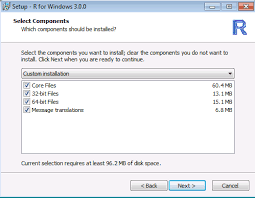
The first thing we need to do is install $\mathrm{R}$, the actual programming language. We will then install RStudio, which is a powerful and user-friendly editor that uses $R$. Throughout this book, we will use $R S t u d i o$, and I will refer to ” $\mathrm{R}$ ” and “RStudio” interchangeably, since we will use $\mathrm{R}$ through $\mathrm{RStudio.}$
- Go to https://rstudio.com and click on “Download RStudio”
- Choose the free version and click “Download”
- Under “Installers”, look for your operating system
You should now have both $R$ and $R$ Studio installed on your computer. If you are a Mac user, you may also want to install XQuartz (https://www.xquartz.org) -you don’t need to do it now, but if you run into problems generating figures or using different graphics packages later on, installing XQuartz is the solution. Because we will use RStudio throughout the book, in the next section, we will explore its interface. Finally, RStudio can also be used online at http:// rstudio.cloud for free (as of August 2020 ), which means you technically don’t need to install anything. That being said, this book (and all its instructions) is based on the desktop version of RStudio, not the cloud version-you can install $\mathrm{R}$ and RStudio and then later use RStudio online as a secondary tool. For reference, the code in this book was last tested using $R$ version 4.0.2 (2020-06-22)_”Taking Off Again” and RStudio Version 1.3.1073 (Mac OS). Therefore, these are the versions on which the coding in this book is based.
统计代写|数据可视化代写Data visualization代考|Interface
Once you have installed both $\mathrm{R}$ and RStudio, open RStudio and click on File $\succ$ New File $\succ$ R Script. Alternatively, press Ctrl $+$ Shift $+\mathrm{N}$ (Windows) or $\mathrm{Cm}+\mathrm{Shift}+\mathrm{N}$ (Mac)-keyboard shortcuts in RStudio are provided in Appendix B. You should now have a screen that looks like Fig. 2.1. Before we explore RStudio’s interface, note that the interface is virtually the same for Mac, Linux, and Windows versions, so while all the examples given in this book are based on the Mac version of RStudio, they also apply to any Linux and Windows versions of RStudio. As a result, every time you see a keyboard shortcut containing Cmd, simply replace that with Ctrl if you are using a Linux or Windows version of RStudio.
What you see in Fig. $2.1$ is that RStudio’s interface revolves around different panes (labeled by dashed circles). Panes B, C, and D were visible when you first opened RStudio-note that their exact location may be slightly different on your RStudio and your operating system. Pane A appeared once you created a new $\mathrm{R}$ script (following the earlier steps). If you look carefully, you will note that a tab called Untitled1 is located at the top of pane A-immediately below the tab you see a group of buttons that include the floppy disk icon for saving documents. Much like your web browser, pane A supports multiple tabs, each of which can contain a file (typically an R script). Each script can contain lines of code, which in turn means that each script can contain an analysis, parts of an analysis, or multiple analyses. If you hit $\mathrm{Cm}+\mathrm{Shift}+\mathrm{N}$ to create another $\mathrm{R}$ Script, another tab will be added to pane A. Next, let’s examine each pane in detail.
Pane A is probably the most important pane in RStudio. This is the pane where we will write our analysis and our comments, that is, this is RStudio’s script window. By the end of this book, we will have written and run several lines of code in pane A. For example, click on pane A and write $2+$ 5. This is your first line of code, that’s why you see 1 on the left margin of pane A. Next, before you hit enter to go to the next line, run that line of code by pressing Cmd + Enter. You can also click on the Run button to the left of Source in Fig. 2.1. You should now see the result of your calculation in pane B: [1] $7 .$
Pane B is RStudio’s console, that is, it is where all your results will be printed. This is where $\mathrm{R}$ will communicate with you. Whereas you will write your questions (in the form of code) in pane A, your answers will appear in pane Bwhen you ran line 1 earlier, you were asking a simple math question in pane $A$ and received the calculated answer in pane B. Finally, note that you can run code directly in pane B. You could, for example, type $2+5$ (or $2+5$ without spaces) in pane B and hit Enter, which would produce the same output as before. You could certainly use pane B for quick calculations and simple tasks, but for an actual analysis with several lines of code and comments,you certainly want the flexibility of pane $A$, which allows you to save your script much like you would save a Word document.
数据可视化代考
统计代写|数据可视化代写Data visualization代考|Why R
R(RCore Team 2020)是一种基于另一种称为 S 的计算机语言的计算机语言。它由 Ross Ihaka 和 Robert Gentlemen 于 1993 年在新西兰创建,是当今使用数据分析的最强大(如果不是最强大)的 tuul 之一。我认为 lhat yuu lave 从来没有听说过你用过 13,因此R未安装在您的计算机上。我还假设您对编程语言几乎没有经验。在本章中,我们将讨论您需要了解的所有内容R理解本书中使用的代码。将建议您阅读其他阅读材料,但您不需要它们来理解接下来的章节中所涵盖的内容。您可能想知道为什么本书没有使用 IBM 的 SPSS,例如,它可能是第二语言研究中最流行的统计工具。如果我们使用谷歌学术引用作为流行度的代表,我们可以清楚地看到 SPSS 在 2010 年之前非常流行(参见 http://r4stats.com/articles/popularity/ 上的报告)。然而,在过去的十年中,其
人气急剧下降。它的限制之一是图形系统低于标准,在各种任务中性能缓慢,以及无法有效处理大型数据集。
使用的原因有几个R进行数据分析是一个明智的决定。一个原因是R是开源的,并拥有大量的在线社区。作为开源,不同的用户可以贡献包R,就像不同的维基百科用户可以为在线百科全书贡献新文章一样。包基本上是我们可以用来完成特定目标的工具(例如,函数)的集合。截至 2020 年 10 月,R有超过 15,000 个包,所以如果您需要在分析中做一些特定的事情,有一个包可以解决这个问题——当然,我们只需要这些包的一小部分。拥有活跃的在线社区也很重要,因为用户可以轻松快速地在论坛帖子中找到帮助。
另一个原因R有利的是它的力量。首先,因为R是一种语言,我们不受一组预先建立的菜单选项或按钮的限制。如果我们希望完成一个目标,无论它多么具体,我们都可以简单地创建自己的函数。SPSS 等典型应用程序具有更加用户友好的图形用户界面 (GUI),但这肯定会限制您可以使用该应用程序做什么。第二,因为R专为数据分析而设计,即使是最新的统计技术也将在其生态系统中可用。因此,无论您需要运行什么类型的模型,R可能会以包裹的形式出现。
统计代写|数据可视化代写Data visualization代考|Installing R and RStudio
我们需要做的第一件事是安装R,实际的编程语言。然后我们将安装 RStudio,它是一个功能强大且用户友好的编辑器,它使用R. 在本书中,我们将使用R小号吨在d一世○, 我会参考”R”和“RStudio”可以互换,因为我们将使用R通过R小号吨在d一世○.
- 转到 https://rstudio.com 并单击“下载 RStudio”
- 选择免费版本并点击“下载”
- 在“安装程序”下,查找您的操作系统
您现在应该同时拥有R和RStudio 安装在您的计算机上。如果您是 Mac 用户,您可能还想安装 XQuartz (https://www.xquartz.org) – 您现在不需要这样做,但如果您以后在生成图形或使用不同的图形包时遇到问题上,安装 XQuartz 是解决方案。因为我们将在整本书中使用 RStudio,所以在下一节中,我们将探索它的界面。最后,还可以在 http://rstudio.cloud 上免费在线使用 RStudio(截至 2020 年 8 月),这意味着您在技术上不需要安装任何东西。话虽如此,这本书(及其所有说明)是基于 RStudio 的桌面版本,而不是云版本——你可以安装R和 RStudio,然后在线使用 RStudio 作为辅助工具。作为参考,本书中的代码最后使用R版本 4.0.2 (2020-06-22)_“再次起飞”和 RStudio 版本 1.3.1073 (Mac OS)。因此,这些是本书编码所基于的版本。
统计代写|数据可视化代写Data visualization代考|Interface
一旦你安装了这两个R和 RStudio,打开 RStudio 并单击文件≻新文件≻R 脚本。或者,按 Ctrl+转移+ñ(Windows) 或C米+小号H一世F吨+ñ(Mac)-RStudio 中的键盘快捷键在附录 B 中提供。您现在应该有一个如图 2.1 所示的屏幕。在我们探索 RStudio 的界面之前,请注意 Mac、Linux 和 Windows 版本的界面实际上是相同的,因此虽然本书中给出的所有示例都基于 RStudio 的 Mac 版本,但它们也适用于任何 Linux 和 Windows 版本RStudio 的。因此,每次您看到包含 Cmd 的键盘快捷键时,如果您使用的是 Linux 或 Windows 版本的 RStudio,只需将其替换为 Ctrl 即可。
你在图中看到的。2.1是 RStudio 的界面围绕不同的窗格(由虚线圆圈标记)旋转。首次打开 RStudio 时可以看到窗格 B、C 和 D – 请注意,它们的确切位置在 RStudio 和操作系统上可能略有不同。一旦您创建了一个新的,窗格 A 就会出现R脚本(按照前面的步骤)。如果你仔细看,你会注意到一个名为 Untitled1 的选项卡位于窗格 A 的顶部——在选项卡的正下方,你会看到一组按钮,其中包括用于保存文档的软盘图标。与您的 Web 浏览器非常相似,窗格 A 支持多个选项卡,每个选项卡都可以包含一个文件(通常是 R 脚本)。每个脚本可以包含代码行,这反过来意味着每个脚本可以包含一个分析、部分分析或多个分析。如果你打C米+小号H一世F吨+ñ创造另一个R脚本,另一个选项卡将添加到窗格 A。接下来,让我们详细检查每个窗格。
窗格 A 可能是 RStudio 中最重要的窗格。这是我们将在其中编写分析和评论的窗格,也就是说,这是 RStudio 的脚本窗口。到本书结束时,我们将在窗格 A 中编写并运行几行代码。例如,单击窗格 A 并编写2+5. 这是您的第一行代码,这就是您在窗格 A 的左边距看到 1 的原因。接下来,在您按 Enter 转到下一行之前,按 Cmd + Enter 运行该行代码。您也可以单击图 2.1 中 Source 左侧的 Run 按钮。您现在应该在窗格 B 中看到计算结果:[1]7.
窗格 B 是 RStudio 的控制台,也就是说,它将打印所有结果。这是哪里R会和你交流。虽然您将在窗格 A 中编写问题(以代码的形式),但您的答案将出现在窗格 B 中当您之前运行第 1 行时,您在窗格中提出了一个简单的数学问题一个并在窗格 B 中收到计算出的答案。最后,请注意,您可以直接在窗格 B 中运行代码。例如,您可以键入2+5(或者2+5没有空格)在窗格 B 中,然后按 Enter,这将产生与以前相同的输出。您当然可以使用窗格 B 进行快速计算和简单任务,但对于具有几行代码和注释的实际分析,您当然需要窗格的灵活性一个,它使您可以像保存 Word 文档一样保存脚本。

统计代写请认准statistics-lab™. statistics-lab™为您的留学生涯保驾护航。
金融工程代写
金融工程是使用数学技术来解决金融问题。金融工程使用计算机科学、统计学、经济学和应用数学领域的工具和知识来解决当前的金融问题,以及设计新的和创新的金融产品。
非参数统计代写
非参数统计指的是一种统计方法,其中不假设数据来自于由少数参数决定的规定模型;这种模型的例子包括正态分布模型和线性回归模型。
广义线性模型代考
广义线性模型(GLM)归属统计学领域,是一种应用灵活的线性回归模型。该模型允许因变量的偏差分布有除了正态分布之外的其它分布。
术语 广义线性模型(GLM)通常是指给定连续和/或分类预测因素的连续响应变量的常规线性回归模型。它包括多元线性回归,以及方差分析和方差分析(仅含固定效应)。
有限元方法代写
有限元方法(FEM)是一种流行的方法,用于数值解决工程和数学建模中出现的微分方程。典型的问题领域包括结构分析、传热、流体流动、质量运输和电磁势等传统领域。
有限元是一种通用的数值方法,用于解决两个或三个空间变量的偏微分方程(即一些边界值问题)。为了解决一个问题,有限元将一个大系统细分为更小、更简单的部分,称为有限元。这是通过在空间维度上的特定空间离散化来实现的,它是通过构建对象的网格来实现的:用于求解的数值域,它有有限数量的点。边界值问题的有限元方法表述最终导致一个代数方程组。该方法在域上对未知函数进行逼近。[1] 然后将模拟这些有限元的简单方程组合成一个更大的方程系统,以模拟整个问题。然后,有限元通过变化微积分使相关的误差函数最小化来逼近一个解决方案。
tatistics-lab作为专业的留学生服务机构,多年来已为美国、英国、加拿大、澳洲等留学热门地的学生提供专业的学术服务,包括但不限于Essay代写,Assignment代写,Dissertation代写,Report代写,小组作业代写,Proposal代写,Paper代写,Presentation代写,计算机作业代写,论文修改和润色,网课代做,exam代考等等。写作范围涵盖高中,本科,研究生等海外留学全阶段,辐射金融,经济学,会计学,审计学,管理学等全球99%专业科目。写作团队既有专业英语母语作者,也有海外名校硕博留学生,每位写作老师都拥有过硬的语言能力,专业的学科背景和学术写作经验。我们承诺100%原创,100%专业,100%准时,100%满意。
随机分析代写
随机微积分是数学的一个分支,对随机过程进行操作。它允许为随机过程的积分定义一个关于随机过程的一致的积分理论。这个领域是由日本数学家伊藤清在第二次世界大战期间创建并开始的。
时间序列分析代写
随机过程,是依赖于参数的一组随机变量的全体,参数通常是时间。 随机变量是随机现象的数量表现,其时间序列是一组按照时间发生先后顺序进行排列的数据点序列。通常一组时间序列的时间间隔为一恒定值(如1秒,5分钟,12小时,7天,1年),因此时间序列可以作为离散时间数据进行分析处理。研究时间序列数据的意义在于现实中,往往需要研究某个事物其随时间发展变化的规律。这就需要通过研究该事物过去发展的历史记录,以得到其自身发展的规律。
回归分析代写
多元回归分析渐进(Multiple Regression Analysis Asymptotics)属于计量经济学领域,主要是一种数学上的统计分析方法,可以分析复杂情况下各影响因素的数学关系,在自然科学、社会和经济学等多个领域内应用广泛。
MATLAB代写
MATLAB 是一种用于技术计算的高性能语言。它将计算、可视化和编程集成在一个易于使用的环境中,其中问题和解决方案以熟悉的数学符号表示。典型用途包括:数学和计算算法开发建模、仿真和原型制作数据分析、探索和可视化科学和工程图形应用程序开发,包括图形用户界面构建MATLAB 是一个交互式系统,其基本数据元素是一个不需要维度的数组。这使您可以解决许多技术计算问题,尤其是那些具有矩阵和向量公式的问题,而只需用 C 或 Fortran 等标量非交互式语言编写程序所需的时间的一小部分。MATLAB 名称代表矩阵实验室。MATLAB 最初的编写目的是提供对由 LINPACK 和 EISPACK 项目开发的矩阵软件的轻松访问,这两个项目共同代表了矩阵计算软件的最新技术。MATLAB 经过多年的发展,得到了许多用户的投入。在大学环境中,它是数学、工程和科学入门和高级课程的标准教学工具。在工业领域,MATLAB 是高效研究、开发和分析的首选工具。MATLAB 具有一系列称为工具箱的特定于应用程序的解决方案。对于大多数 MATLAB 用户来说非常重要,工具箱允许您学习和应用专业技术。工具箱是 MATLAB 函数(M 文件)的综合集合,可扩展 MATLAB 环境以解决特定类别的问题。可用工具箱的领域包括信号处理、控制系统、神经网络、模糊逻辑、小波、仿真等。