如果你也在 怎样代写最优控制optimal control这个学科遇到相关的难题,请随时右上角联系我们的24/7代写客服。
最优控制是为一个动态系统确定一段时期内的控制和状态轨迹,以使性能指数最小化的过程。
statistics-lab™ 为您的留学生涯保驾护航 在代写最优控制optimal control方面已经树立了自己的口碑, 保证靠谱, 高质且原创的统计Statistics代写服务。我们的专家在代写最优控制optimal control代写方面经验极为丰富,各种代写最优控制Soptimal control相关的作业也就用不着说。
我们提供的最优控制optimal control及其相关学科的代写,服务范围广, 其中包括但不限于:
- Statistical Inference 统计推断
- Statistical Computing 统计计算
- Advanced Probability Theory 高等楖率论
- Advanced Mathematical Statistics 高等数理统计学
- (Generalized) Linear Models 广义线性模型
- Statistical Machine Learning 统计机器学习
- Longitudinal Data Analysis 纵向数据分析
- Foundations of Data Science 数据科学基础
统计代写|最优控制作业代写optimal control代考|Basic Concepts and Definitions
We will use the word system as a primitive term in this book. The only property that we require of a system is that it is capable of existing in various states. Let the (real) variable $x(t)$ be the state variable of the system at time $t \in[0, T]$, where $T>0$ is a specified time horizon for the system under consideration. For example, $x(t)$ could measure the inventory level at time $t$, the amount of advertising goodwill at time $t$, or the amount of unconsumed wealth or natural resources at time $t$.
We assume that there is a way of controlling the state of the system. Let the (real) variable $u(t)$ be the control variable of the system at time $t$. For example, $u(t)$ could be the production rate at time $t$, the advertising rate at time $t$, etc.
Given the values of the state variable $x(t)$ and the control variable $u(t)$ at time $t$, the state equation, a differential equation,
$$
\dot{x}(t)=f(x(t), u(t), t), \quad x(0)=x_{0},
$$
specifies the instantaneous rate of change in the state variable, where $\dot{x}(t)$ is a commonly used notation for $d x(t) / d t, f$ is a given function of $x, u$, and $t$, and $x_{0}$ is the initial value of the state variable. If we know the initial value $x_{0}$ and the control trajectory, i.e., the values of $u(t)$ over the whole time interval $0 \leq t \leq T$, then we can integrate (1.1) to get the state trajectory, i.e., the values of $x(t)$ over the same time interval. We want to choose the control trajectory so that the state and control trajectories maximize the objective functional, or simply the objective function,
$$
J=\int_{0}^{T} F(x(t), u(t), t) d t+S[x(T), T]
$$
In (1.2), $F$ is a given function of $x, u$, and $t$, which could measure the benefit minus the cost of advertising, the utility of consumption, the negative of the cost of inventory and production, etc. Also in (1.2), the function $S$ gives the salvage value of the ending state $x(T)$ at time $T$. The salvage value is needed so that the solution will make “good sense” at the end of the horizon.
统计代写|最优控制作业代写optimal control代考|Formulation of Simple Control Models
We now formulate three simple models chosen from the areas of production, advertising, and economics. Our only objective here is to identify and interpret in these models each of the variables and functions described in the previous section. The solutions for each of these models will be given in detail in later chapters.
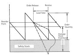
Example 1.1 A Production-Inventory Model. The various quantities that define this model are summarized in Table $1.1$ for easy comparison with the other models that rulluw.
We consider the production and inventory storage of a given good, such as steel, in order to meet an exogenous demand. The state variable $I(t)$ measures the number of tons of steel that we have on hand at time $t \in[0, T]$. There is an exogenous demand rate $S(t)$ tons of steel per day at time $t \in[0, T]$, and we must choose the production rate $P(t)$ tons of steel per day at time $t \in[0, T]$. Given the initial inventory of $I_{0}$ tons of steel on hand at $t=0$, the state equation
$$
\dot{I}(t)=P(t)-S(t)
$$
describes how the steel inventory changes over time. Since $h(I)$ is the cost of holding inventory $I$ in dollars per day, and $c(P)$ is the cost of producing steel at rate $P$, also in dollars per day, the objective function is to maximize the negative of the sum of the total holding and production costs over the period of $T$ days. Of course, maximizing the negative sum is the same as minimizing the sum of holding and production costs. The state variable constraint, $I(t) \geq 0$, is imposed so that the demand is satisfied for all $t$. In other words, backlogging of demand is not permitted. (An alternative formulation is to make $h(I)$ become very large when $I$ becomes negative, i.e., to impose a stockout penalty cost.) The control constraints keep the production rate $P(t)$ between a specified lower bound $P_{\min }$ and a specified upper bound $P_{\max }$. Finally, the terminal constraint $I(T) \geq I_{\min }$ is imposed so that the terminal inventory is at least $I_{\min }$.
The statement of the problem is lengthy because of the number of variables, functions, and parameters which are involved. However, with the production and inventory interpretations as given, it is not difficult to see the reasons for each condition. In Chap. 6, various versions of this model will be solved in detail. In Sect. $12.2$, we will deal with a stochastic version of this model.
最优控制代考
统计代写|最优控制作业代写optimal control代考|Basic Concepts and Definitions
在本书中,我们将使用系统一词作为原始术语。我们要求系统的唯一属性是它能够以各种状态存在。让 (实际) 变 量 $x(t)$ 是系统在某一时刻的状态变量 $t \in[0, T]$ ,在哪里 $T>0$ 是所考虑系统的指定时间范围。例如, $x(t)$ 可以 及时测量库存水平 $t$ ,当时的广告商誉金额 $t$ ,或当时末消耗的财富或自然资源的数量 $t$.
我们假设有一种方法可以控制系统的状态。让 (实际) 变量 $u(t)$ 是系统在时间的控制变量 $t$. 例如, $u(t)$ 可能是当时 的生产率 $t$ ,当时的广告费率 ,ETC。
给定状态变量的值 $x(t)$ 和控制变量 $u(t)$ 有时 $t$ ,状态方程,微分方程,
$$
\dot{x}(t)=f(x(t), u(t), t), \quad x(0)=x_{0},
$$
指定状态变量的瞬时变化率,其中 $\dot{x}(t)$ 是一种常用的表示法 $d x(t) / d t, f$ 是一个给定的函数 $x, u$ ,和 $t$ ,和 $x_{0}$ 是状 态变量的初始值。如果我们知道初始值 $x_{0}$ 和控制轨迹,即 $u(t)$ 在整个时间间隔内 $0 \leq t \leq T$ ,那么我们可以对 (1.1)进行积分得到状态轨迹,即 $x(t)$ 在同一时间间隔内。我们要选择控制轨迹,使状态和控制轨迹最大化目标函 数,或者简単地目标函数,
$$
J=\int_{0}^{T} F(x(t), u(t), t) d t+S[x(T), T]
$$
在 $(1.2)$ 中, $F$ 是一个给定的函数 $x, u$ ,和 $t$ ,它可以衡量收益减去广告成本、消费效用、库存和生产成本的负数 等。同样在 (1.2) 中,函数 $S$ 给出结束状态的残值 $x(T)$ 有时 $T$. 残值是必需的,这样解决方案才能在地平线的尽头 产生“良好的意义”。
统计代写|最优控制作业代写optimal control代考|Formulation of Simple Control Models
我们现在制定从生产、广告和经济领域中选择的三个简单模型。我们在这里的唯一目标是在这些模型中识别和解释 上一节中描述的每个变量和函数。这些模型中的每一个的解决方案将在后面的章节中详细给出。 示例 $1.1$ 生产库存模型。表中总结了定义此模型的各种量 $1.1$ 以便与其他 ruluw 模型进行比较。
我们考虑给定商品 (如钢铁) 的生产和库存,以满足外生需求。状态变量 $I(t)$ 衡量我们当时手头的钢材吨数 $t \in[0, T]$. 存在外生需求率 $S(t)$ 每天多少吨钢 $t \in[0, T]$ ,我们必须选择生产率 $P(t)$ 每天多少吨钢 $t \in[0, T]$. 鉴 于初始库存 $I_{0}$ 吨钢在手 $t=0$, 状态方程
$$
\dot{I}(t)=P(t)-S(t)
$$
描述钢铁库存如何随时间变化。自从 $h(I)$ 是持有库存的成本 $I$ 每天以美元计,以及 $c(P)$ 是按速率生产钢铁的成本 $P$ ,同样以美元/天为单位,目标函数是使总持有成本和生产成本之和的负值最大化 $T$ 天。当然,最大化负总和与最 小化持有成本和生产成本的总和是一样的。状态变量约束, $I(t) \geq 0$ ,是为了满足所有人的需求 $t$. 换言之,不允许 积压需求。(另一种公式是使 $h(I)$ 当变得非常大 $I$ 变为负数,即施加缺货惩罚成本。)控制约束保持生产率 $P(t)$ 在指定的下限之间 $P_{\min }$ 和一个指定的上限 $P_{\max }$. 最后,终端约束 $I(T) \geq I_{\min }$ 强制使终端库存至少为 $I_{\min }$.
由于涉及的变量、函数和参数的数量,问题的陈述很长。但是,根据给定的生产和库存解释,不难看出每种情况的 原因。在第一章。6、这个模型的各个版本都会详细解决。昆虫。12.2,我们将处理这个模型的随机版本。

统计代写请认准statistics-lab™. statistics-lab™为您的留学生涯保驾护航。
金融工程代写
金融工程是使用数学技术来解决金融问题。金融工程使用计算机科学、统计学、经济学和应用数学领域的工具和知识来解决当前的金融问题,以及设计新的和创新的金融产品。
非参数统计代写
非参数统计指的是一种统计方法,其中不假设数据来自于由少数参数决定的规定模型;这种模型的例子包括正态分布模型和线性回归模型。
广义线性模型代考
广义线性模型(GLM)归属统计学领域,是一种应用灵活的线性回归模型。该模型允许因变量的偏差分布有除了正态分布之外的其它分布。
术语 广义线性模型(GLM)通常是指给定连续和/或分类预测因素的连续响应变量的常规线性回归模型。它包括多元线性回归,以及方差分析和方差分析(仅含固定效应)。
有限元方法代写
有限元方法(FEM)是一种流行的方法,用于数值解决工程和数学建模中出现的微分方程。典型的问题领域包括结构分析、传热、流体流动、质量运输和电磁势等传统领域。
有限元是一种通用的数值方法,用于解决两个或三个空间变量的偏微分方程(即一些边界值问题)。为了解决一个问题,有限元将一个大系统细分为更小、更简单的部分,称为有限元。这是通过在空间维度上的特定空间离散化来实现的,它是通过构建对象的网格来实现的:用于求解的数值域,它有有限数量的点。边界值问题的有限元方法表述最终导致一个代数方程组。该方法在域上对未知函数进行逼近。[1] 然后将模拟这些有限元的简单方程组合成一个更大的方程系统,以模拟整个问题。然后,有限元通过变化微积分使相关的误差函数最小化来逼近一个解决方案。
tatistics-lab作为专业的留学生服务机构,多年来已为美国、英国、加拿大、澳洲等留学热门地的学生提供专业的学术服务,包括但不限于Essay代写,Assignment代写,Dissertation代写,Report代写,小组作业代写,Proposal代写,Paper代写,Presentation代写,计算机作业代写,论文修改和润色,网课代做,exam代考等等。写作范围涵盖高中,本科,研究生等海外留学全阶段,辐射金融,经济学,会计学,审计学,管理学等全球99%专业科目。写作团队既有专业英语母语作者,也有海外名校硕博留学生,每位写作老师都拥有过硬的语言能力,专业的学科背景和学术写作经验。我们承诺100%原创,100%专业,100%准时,100%满意。
随机分析代写
随机微积分是数学的一个分支,对随机过程进行操作。它允许为随机过程的积分定义一个关于随机过程的一致的积分理论。这个领域是由日本数学家伊藤清在第二次世界大战期间创建并开始的。
时间序列分析代写
随机过程,是依赖于参数的一组随机变量的全体,参数通常是时间。 随机变量是随机现象的数量表现,其时间序列是一组按照时间发生先后顺序进行排列的数据点序列。通常一组时间序列的时间间隔为一恒定值(如1秒,5分钟,12小时,7天,1年),因此时间序列可以作为离散时间数据进行分析处理。研究时间序列数据的意义在于现实中,往往需要研究某个事物其随时间发展变化的规律。这就需要通过研究该事物过去发展的历史记录,以得到其自身发展的规律。
回归分析代写
多元回归分析渐进(Multiple Regression Analysis Asymptotics)属于计量经济学领域,主要是一种数学上的统计分析方法,可以分析复杂情况下各影响因素的数学关系,在自然科学、社会和经济学等多个领域内应用广泛。
MATLAB代写
MATLAB 是一种用于技术计算的高性能语言。它将计算、可视化和编程集成在一个易于使用的环境中,其中问题和解决方案以熟悉的数学符号表示。典型用途包括:数学和计算算法开发建模、仿真和原型制作数据分析、探索和可视化科学和工程图形应用程序开发,包括图形用户界面构建MATLAB 是一个交互式系统,其基本数据元素是一个不需要维度的数组。这使您可以解决许多技术计算问题,尤其是那些具有矩阵和向量公式的问题,而只需用 C 或 Fortran 等标量非交互式语言编写程序所需的时间的一小部分。MATLAB 名称代表矩阵实验室。MATLAB 最初的编写目的是提供对由 LINPACK 和 EISPACK 项目开发的矩阵软件的轻松访问,这两个项目共同代表了矩阵计算软件的最新技术。MATLAB 经过多年的发展,得到了许多用户的投入。在大学环境中,它是数学、工程和科学入门和高级课程的标准教学工具。在工业领域,MATLAB 是高效研究、开发和分析的首选工具。MATLAB 具有一系列称为工具箱的特定于应用程序的解决方案。对于大多数 MATLAB 用户来说非常重要,工具箱允许您学习和应用专业技术。工具箱是 MATLAB 函数(M 文件)的综合集合,可扩展 MATLAB 环境以解决特定类别的问题。可用工具箱的领域包括信号处理、控制系统、神经网络、模糊逻辑、小波、仿真等。