如果你也在 怎样代写机器学习machine learning这个学科遇到相关的难题,请随时右上角联系我们的24/7代写客服。
机器学习是一种数据分析的方法,可以自动建立分析模型。它是人工智能的一个分支,其基础是系统可以从数据中学习,识别模式,并在最小的人为干预下做出决定。
statistics-lab™ 为您的留学生涯保驾护航 在代写机器学习machine learning方面已经树立了自己的口碑, 保证靠谱, 高质且原创的统计Statistics代写服务。我们的专家在代写机器学习machine learning方面经验极为丰富,各种代写机器学习machine learning相关的作业也就用不着说。
我们提供的机器学习machine learning及其相关学科的代写,服务范围广, 其中包括但不限于:
- Statistical Inference 统计推断
- Statistical Computing 统计计算
- Advanced Probability Theory 高等楖率论
- Advanced Mathematical Statistics 高等数理统计学
- (Generalized) Linear Models 广义线性模型
- Statistical Machine Learning 统计机器学习
- Longitudinal Data Analysis 纵向数据分析
- Foundations of Data Science 数据科学基础

统计代写|机器学习作业代写machine learning代考|The Single-Attribute Case
Let us start with something so simple as to be almost unrealistic: a domain where each example is described with a single attribute. Once we have grasped the principles of Bayesian classifiers under these simplified circumstances, we will generalize the idea for more realistic settings.
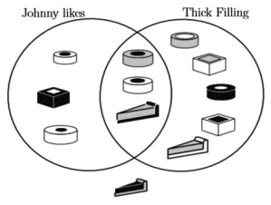
Prior probability and conditional probability. Let us return to the toy domain from the previous chapter. The training set consists of twelve pies ( $N_{a l l}=12$ ), of which six are positive examples of the given class $\left(N_{p a s}=6\right)$ and six are negative $\left(N_{\text {neg }}=6\right)$. Assuming that the examples represent faithfully the given domain, the probability of Johnny liking a randomly picked pie is fifty percent because fifty percent of the training examples are positive.
$$
P(\mathrm{pos})=\frac{N_{p o s}}{N_{a l l}}=\frac{6}{12}=0.5
$$
Let us now choose one of the attributes, say, filling-size. The training set contains eight examples with thick filling $\left(N_{\text {thick }}=8\right)$, of which three are labeled as positive $\left(N_{\text {pos } \mid \text { shick }}=3\right.$ ). We say that the conditional probability of an example being positive given that $f i l$ ing – si ze =thick is $37.5 \%$ : the relative frequency of positive examples among those with thick filling indicates:
$$
P(\mathrm{pos} \mid \text { thick })=\frac{N_{\text {pos } \mid \text { hick }}}{N_{\text {thick }}}=\frac{3}{8}=0.375
$$
统计代写|机器学习作业代写machine learning代考|Vectors of Discrete Attributes
Let us now proceed to a simple way of using the Bayes formula in more realistic domains where the examples are described by vectors of attributes such as $\mathbf{x}=$ $\left(x_{1}, x_{2}, \ldots, x_{n}\right)$, and where there are more than two classes.
Multiple Classes Many realistic applications are marked by more than two classes, not just the pos and neg from the “pies” domain. If $c_{l}$ is the label of the $i$-th class, and if $\mathbf{x}$ is the vector describing the object we want to classify, the Bayes formula acquires the following form:
$$
P\left(c_{i} \mid \mathbf{x}\right)=\frac{P\left(\mathbf{x} \mid c_{i}\right) P\left(c_{i}\right)}{P(\mathbf{x})}
$$
The denominator being the same for each class, we choose the class that maximizes the numerator, $P\left(\mathbf{x} \mid c_{i}\right) P\left(c_{i}\right)$. Here, $P\left(c_{i}\right)$ is estimated by the relative frequency of $c_{i}$ in the training set. With $P\left(\mathbf{x} \mid c_{i}\right)$, however, things are not so simple.
A Vector’s Probability $P\left(\mathbf{x} \mid c_{i}\right)$ is the probability that a randomly selected instance of class $c_{l}$ is described by vector $\mathbf{x}$. Can the value of this probability be estimated by relative frequency? Not really. In the “pies” domain, the size of the instance space was 108 different examples, of which the training set contained twelve, while none of the other vectors (the vast majority!) was represented at all. Relative frequency would indicate that the probability of $\mathbf{x}$ being positive is $P(\mathbf{x} \mid$ pos $)=1 / 6$ if we find $\mathbf{x}$ among the positive training examples, and $P(\mathbf{x} \mid \mathrm{pos})=0$ if we do not. In other words, any $\mathbf{x}$ identical to some training example “inherits” this example’s class label; if the vector is not in the training set, we have $P\left(\mathbf{x} \mid c_{i}\right)=0$ for any $c_{i}$. In this case, the numerator in the Bayes formula will always be $P\left(\mathbf{x} \mid c_{i}\right) P\left(c_{i}\right)=0$, which makes
it impossible for us to choose the most probable class. Evidently, we are not getting very far trying to calculate the probability of an event that occurs only once-if it occurs at all.
The situation improves if only individual attributes are considered. For instance, shape=circle occurs four times among the positive examples and twice among the negative, the corresponding probabilities thus being $P($ shape $=$ circle|pos $)=4 / 6$ and $P($ shape $=$ circle $\mid$ neg $)=2 / 6$. We see that, if an attribute can acquire only two or three values, chances are high that each of these values is represented in the training set more than once, thus providing better grounds for probability estimates.
统计代写|机器学习作业代写machine learning代考|Rare Events: An Expert’s Intuition
For simplicity, probability is often estimated by relative frequency. Having observed phenomenon $x$ thirty times in one hundred trials, we conclude that its probability is $P(x)=0.3$. This is how we did it in the previous sections.
Estimates of this kind, however, can be trusted only when based on a great many observations. While it is conceivable that a coin flipped four times comes up heads three times, it would be silly to jump to the conclusion that $P$ (heads) $=0.75$. The physical nature of the experiment suggests otherwise: a fair coin should come up heads fifty percent of the time. Can this prior expectation help us improve our probability estimates in domains with few observations?
The answer is yes. Prior expectations are employed in the so-called $m$-estimates.
Essence of $m$-Estimates Let us consider experiments with a coin that may be fairor unfair. In the absence of any extra information, our estimate of the probability of heads will be $\pi_{\text {heads }}=0.5$. But how confident are we in this estimate? This is quantified by an auxiliary parameter, $m$, that informs the class-predicting program about the amount of our uncertainty. The higher the value of $m$, the more the probability estimate, $\pi_{\text {head }}=0.5$, is to be trusted.
Returning to our experimental coin-flipping, let us denote by $N_{a l l}$ the total number of trials, and by $N_{\text {heads }}$ the number of “heads” observed in these trials. The following formula combines these values with the prior estimate and with our confidence in this estimate’s reliability:
$$
P_{\text {heads }}=\frac{N_{\text {heads }}+m \pi_{\text {heads }}}{N_{a l l}+m}
$$
Note that the formula degenerates to the prior estimate if no experimental evidence has yet been accumulated, in which case, $P_{\text {heads }}=\pi_{\text {heads }}$ because $N_{a l l}=N_{\text {heads }}=$ 0 . Conversely, the formula converges to that of relative frequency if $N_{a l l}$ and $N_{\text {heads }}$ are so big as to render negligible the terms $m \pi_{h e a d s}$ and $m$.
With $\pi_{\text {heads }}=0.5$ and $m=2$, we obtain the following:
$$
P_{\text {heads }}=\frac{N_{\text {heads }}+2 \times 0.5}{N_{a l l}+2}=\frac{N_{\text {heads }}+1}{N_{a l l}+2}
$$
机器学习代写
统计代写|机器学习作业代写machine learning代考|The Single-Attribute Case
让我们从简单到几乎不切实际的东西开始:每个示例都用一个属性描述的域。一旦我们在这些简化的情况下掌握了贝叶斯分类器的原理,我们将把这个想法推广到更现实的设置中。
先验概率和条件概率。让我们从上一章回到玩具领域。训练集由十二个饼图(ñ一种ll=12),其中六个是给定类的正例(ñp一种s=6)六个是负数(ñ否定 =6). 假设这些例子忠实地代表了给定的领域,约翰尼喜欢一个随机挑选的馅饼的概率是百分之五十,因为百分之五十的训练例子是正面的。
磷(p这s)=ñp这sñ一种ll=612=0.5
现在让我们选择其中一个属性,比如填充大小。训练集包含八个厚填充的示例(ñ厚的 =8),其中三个被标记为阳性(ñ位置 ∣ 鸡肋 =3)。我们说一个例子的条件概率是正的,给定F一世ling – 大小 = 厚是37.5%:填充厚实的正例的相对频率表明:
磷(p这s∣ 厚的 )=ñ位置 ∣ 希克 ñ厚的 =38=0.375
统计代写|机器学习作业代写machine learning代考|Vectors of Discrete Attributes
现在让我们继续在更现实的领域中使用贝叶斯公式的简单方法,其中示例由属性向量描述,例如X= (X1,X2,…,Xn), 并且有两个以上的类。
多个类 许多实际应用程序都由两个以上的类标记,而不仅仅是“派”域中的 pos 和 neg。如果Cl是标签一世-th 类,如果X是描述我们要分类的对象的向量,贝叶斯公式得到如下形式:
磷(C一世∣X)=磷(X∣C一世)磷(C一世)磷(X)
每个类别的分母相同,我们选择使分子最大化的类别,磷(X∣C一世)磷(C一世). 这里,磷(C一世)由相对频率估计C一世在训练集中。和磷(X∣C一世)然而,事情并没有那么简单。
向量的概率磷(X∣C一世)是随机选择的类实例的概率Cl由向量描述X. 这个概率的值可以通过相对频率来估计吗?并不真地。在“派”域中,实例空间的大小为 108 个不同的示例,其中训练集包含 12 个,而其他向量(绝大多数!)根本没有表示。相对频率表明X积极是磷(X∣位置)=1/6如果我们发现X在积极的训练样本中,以及磷(X∣p这s)=0如果我们不这样做。换句话说,任何X与某些训练示例相同,“继承”该示例的类标签;如果向量不在训练集中,我们有磷(X∣C一世)=0对于任何C一世. 在这种情况下,贝叶斯公式中的分子总是磷(X∣C一世)磷(C一世)=0,这使得
我们不可能选择最可能的类别。显然,我们并没有走得太远,试图计算一个事件只发生一次的概率——如果它发生的话。
如果只考虑个别属性,情况会有所改善。例如,shape=circle 在正例中出现四次,在负例中出现两次,因此相应的概率为磷(形状=圈子|位置)=4/6和磷(形状=圆圈∣否定)=2/6. 我们看到,如果一个属性只能获得两个或三个值,那么这些值中的每一个都很有可能在训练集中多次表示,从而为概率估计提供了更好的基础。
统计代写|机器学习作业代写machine learning代考|Rare Events: An Expert’s Intuition
为简单起见,概率通常通过相对频率来估计。观察到现象X一百次试验三十次,我们得出结论,它的概率是磷(X)=0.3. 这就是我们在前面几节中的做法。
然而,这种估计只有在基于大量观察时才能被信任。虽然可以想象一枚硬币被抛了四次,正面朝上 3 次,但贸然下结论是愚蠢的磷(头)=0.75. 实验的物理性质表明并非如此:一枚公平的硬币应该有百分之五十的时间出现正面。这种先验期望能否帮助我们改进在观察很少的领域中的概率估计?
答案是肯定的。在所谓的米-估计。
精华米- 估计让我们考虑使用可能公平或不公平的硬币进行的实验。在没有任何额外信息的情况下,我们对正面概率的估计将是圆周率头 =0.5. 但我们对这个估计有多大信心?这是由一个辅助参数量化的,米,这会告知类别预测程序我们不确定性的数量。的价值越高米,概率估计越多,圆周率头 =0.5, 是值得信赖的。
回到我们的实验掷硬币,让我们表示ñ一种ll试验的总数,并由ñ头 在这些试验中观察到的“头”的数量。以下公式将这些值与先前的估计以及我们对该估计的可靠性的信心相结合:
磷头 =ñ头 +米圆周率头 ñ一种ll+米
请注意,如果尚未积累实验证据,则该公式会退化为先前的估计,在这种情况下,磷头 =圆周率头 因为ñ一种ll=ñ头 =0 . 相反,如果该公式收敛于相对频率的公式ñ一种ll和ñ头 大到可以忽略不计的条款米圆周率H和一种ds和米.
和圆周率头 =0.5和米=2,我们得到以下信息:
磷头 =ñ头 +2×0.5ñ一种ll+2=ñ头 +1ñ一种ll+2

统计代写请认准statistics-lab™. statistics-lab™为您的留学生涯保驾护航。统计代写|python代写代考
随机过程代考
在概率论概念中,随机过程是随机变量的集合。 若一随机系统的样本点是随机函数,则称此函数为样本函数,这一随机系统全部样本函数的集合是一个随机过程。 实际应用中,样本函数的一般定义在时间域或者空间域。 随机过程的实例如股票和汇率的波动、语音信号、视频信号、体温的变化,随机运动如布朗运动、随机徘徊等等。
贝叶斯方法代考
贝叶斯统计概念及数据分析表示使用概率陈述回答有关未知参数的研究问题以及统计范式。后验分布包括关于参数的先验分布,和基于观测数据提供关于参数的信息似然模型。根据选择的先验分布和似然模型,后验分布可以解析或近似,例如,马尔科夫链蒙特卡罗 (MCMC) 方法之一。贝叶斯统计概念及数据分析使用后验分布来形成模型参数的各种摘要,包括点估计,如后验平均值、中位数、百分位数和称为可信区间的区间估计。此外,所有关于模型参数的统计检验都可以表示为基于估计后验分布的概率报表。
广义线性模型代考
广义线性模型(GLM)归属统计学领域,是一种应用灵活的线性回归模型。该模型允许因变量的偏差分布有除了正态分布之外的其它分布。
statistics-lab作为专业的留学生服务机构,多年来已为美国、英国、加拿大、澳洲等留学热门地的学生提供专业的学术服务,包括但不限于Essay代写,Assignment代写,Dissertation代写,Report代写,小组作业代写,Proposal代写,Paper代写,Presentation代写,计算机作业代写,论文修改和润色,网课代做,exam代考等等。写作范围涵盖高中,本科,研究生等海外留学全阶段,辐射金融,经济学,会计学,审计学,管理学等全球99%专业科目。写作团队既有专业英语母语作者,也有海外名校硕博留学生,每位写作老师都拥有过硬的语言能力,专业的学科背景和学术写作经验。我们承诺100%原创,100%专业,100%准时,100%满意。
机器学习代写
随着AI的大潮到来,Machine Learning逐渐成为一个新的学习热点。同时与传统CS相比,Machine Learning在其他领域也有着广泛的应用,因此这门学科成为不仅折磨CS专业同学的“小恶魔”,也是折磨生物、化学、统计等其他学科留学生的“大魔王”。学习Machine learning的一大绊脚石在于使用语言众多,跨学科范围广,所以学习起来尤其困难。但是不管你在学习Machine Learning时遇到任何难题,StudyGate专业导师团队都能为你轻松解决。
多元统计分析代考
基础数据: $N$ 个样本, $P$ 个变量数的单样本,组成的横列的数据表
变量定性: 分类和顺序;变量定量:数值
数学公式的角度分为: 因变量与自变量
时间序列分析代写
随机过程,是依赖于参数的一组随机变量的全体,参数通常是时间。 随机变量是随机现象的数量表现,其时间序列是一组按照时间发生先后顺序进行排列的数据点序列。通常一组时间序列的时间间隔为一恒定值(如1秒,5分钟,12小时,7天,1年),因此时间序列可以作为离散时间数据进行分析处理。研究时间序列数据的意义在于现实中,往往需要研究某个事物其随时间发展变化的规律。这就需要通过研究该事物过去发展的历史记录,以得到其自身发展的规律。
回归分析代写
多元回归分析渐进(Multiple Regression Analysis Asymptotics)属于计量经济学领域,主要是一种数学上的统计分析方法,可以分析复杂情况下各影响因素的数学关系,在自然科学、社会和经济学等多个领域内应用广泛。
MATLAB代写
MATLAB 是一种用于技术计算的高性能语言。它将计算、可视化和编程集成在一个易于使用的环境中,其中问题和解决方案以熟悉的数学符号表示。典型用途包括:数学和计算算法开发建模、仿真和原型制作数据分析、探索和可视化科学和工程图形应用程序开发,包括图形用户界面构建MATLAB 是一个交互式系统,其基本数据元素是一个不需要维度的数组。这使您可以解决许多技术计算问题,尤其是那些具有矩阵和向量公式的问题,而只需用 C 或 Fortran 等标量非交互式语言编写程序所需的时间的一小部分。MATLAB 名称代表矩阵实验室。MATLAB 最初的编写目的是提供对由 LINPACK 和 EISPACK 项目开发的矩阵软件的轻松访问,这两个项目共同代表了矩阵计算软件的最新技术。MATLAB 经过多年的发展,得到了许多用户的投入。在大学环境中,它是数学、工程和科学入门和高级课程的标准教学工具。在工业领域,MATLAB 是高效研究、开发和分析的首选工具。MATLAB 具有一系列称为工具箱的特定于应用程序的解决方案。对于大多数 MATLAB 用户来说非常重要,工具箱允许您学习和应用专业技术。工具箱是 MATLAB 函数(M 文件)的综合集合,可扩展 MATLAB 环境以解决特定类别的问题。可用工具箱的领域包括信号处理、控制系统、神经网络、模糊逻辑、小波、仿真等。