如果你也在 怎样代写生物统计biostatistics这个学科遇到相关的难题,请随时右上角联系我们的24/7代写客服。
生物统计学是将统计技术应用于健康相关领域的科学研究,包括医学、生物学和公共卫生,并开发新的工具来研究这些领域。
statistics-lab™ 为您的留学生涯保驾护航 在代写生物统计biostatistics方面已经树立了自己的口碑, 保证靠谱, 高质且原创的统计Statistics代写服务。我们的专家在代写生物统计biostatistics代写方面经验极为丰富,各种生物统计biostatistics相关的作业也就用不着说。
我们提供的生物统计biostatistics及其相关学科的代写,服务范围广, 其中包括但不限于:
- Statistical Inference 统计推断
- Statistical Computing 统计计算
- Advanced Probability Theory 高等概率论
- Advanced Mathematical Statistics 高等数理统计学
- (Generalized) Linear Models 广义线性模型
- Statistical Machine Learning 统计机器学习
- Longitudinal Data Analysis 纵向数据分析
- Foundations of Data Science 数据科学基础
统计代写|生物统计代写biostatistics代考|Flexible Distributions: The Skew-t Case
In the context of distribution theory, a central theme is the study of flexible parametric families of probability distributions, that is, families allowing substantial variation of their behaviour when the parameters span their admissible range.
For brevity, we shall refer to this domain with the phrase ‘flexible distributions’. The archetypal construction of this logic is represented by the Pearson system of curves for univariate continuous variables. In this formulation, the density function is regulated by four parameters, allowing wide variation of the measures of skewness and kurtosis, hence providing much more flexibility than in the basic case represented by the normal distribution, where only location and scale can be adjusted.
Since Pearson times, flexible distributions have remained a persistent theme of interest in the literature, with a particularly intense activity in recent years. A prominen feature of newer developments is the increased sonsideration for multivariate distributions, reflecting the current availability in applied work of larger datasets, both in sample size and in dimensionality. In the multivariate setting, the various formulations often feature four blocks of parameters to regulate location, scale, skewness and kurtosis.
While providing powerful tools for data fitting, flexible distributions also pose some challenges when we enter the concrete estimation stage. We shall be working with maximum likelihood estimation (MLE) or variants of it, but qualitatively similar issues exist for other criteria. Explicit expressions of the estimates are out of the question; some numerical optimization procedure is always involved and this process is not so trivial because of the larger number of parameters involved, as compared with fitting simpler parametric models, such as a Gamma or a Beta distribution. Furthermore, in some circumstances, the very flexibility of these parametric families can lead to difficulties: if the data pattern does not aim steadily towards a certain point of the parameter space, there could be two or more such points which constitute comparably valid candidates in terms of log-likelihood or some other estimation criterion. Clearly, these problems are more challenging with small sample size, later denoted $n$, since the log-likelihood function (possibly tuned by a prior distribution) is relatively more flat, but numerical experience has shown that they can persist even for fairly large $n$, in certain cases.
统计代写|生物统计代写biostatistics代考|The Skew-t Distribution: Basic Facts
Before entering our actual development, we recall some basic facts about the ST parametric family of continuous distributions. In its simplest description, it is obtained as a perturbation of the classical Student’s $t$ distribution. For a more specific description, start from the univariate setting, where the components of the family are identified by four parameters. Of these four parameters, the one denoted $\xi$ in the following regulates the location of the distribution; scale is regulated by the positive parameter $\omega$; shape (representing departure from symmetry) is regulated by $\lambda$; tail-weight is regulated by $v$ (with $v>0$ ), denoted ‘degrees of freedom’ like for a classical $t$ distribution.
It is convenient to introduce the distribution in the ‘standard case’, that is, with location $\xi=0$ and scale $\omega=1$. In this case, the density function is
$$
t(z ; \lambda, v)=2 t(z ; v) T\left(\lambda z \sqrt{\frac{v+1}{v+z^{2}}} ; v+1\right), \quad z \in \mathbb{R}
$$
where
$$
t(z ; v)=\frac{\Gamma\left(\frac{1}{2}(v+1)\right)}{\sqrt{\pi v} \Gamma\left(\frac{1}{2} v\right)}\left(1+\frac{z^{2}}{v}\right)^{-(v+1) / 2}, \quad z \in \mathbb{R}
$$
is the density function of the classical Student’s $t$ on $v$ degrees of freedom and $T(\cdot ; v)$ denotes its distribution function; note however that in (1) this is evaluated with $v+1$ degrees of freedom. Also, note that the symbol $t$ is used for both densities in (1) and (2), which are distinguished by the presence of either one or two parameters.
If $Z$ is a random variable with density function (1), the location and scale transform $Y=\xi+\omega Z$ has density function
$$
t_{Y}(x ; \theta)=\omega^{-1} t(z ; \lambda, v), \quad z=\omega^{-1}(x-\xi),
$$
where $\theta=(\xi, \omega, \lambda, v)$. In this case, we write $Y \sim \operatorname{ST}\left(\xi, \omega^{2}, \lambda, v\right)$, where $\omega$ is squared for similarity with the usual notation for normal distributions.
When $\lambda=0$, we recover the scale-and-location family generated by the $t$ distribution (2). When $v \rightarrow \infty$, we obtain the skew-normal (SN) distribution with parameters $(\xi, \omega, \lambda)$, which is described for instance by Azzalini and Capitanio (2014, Chap. 2). When $\lambda=0$ and $v \rightarrow \infty$, (3) converges to the $\mathrm{N}\left(\xi, \omega^{2}\right)$ distribution.
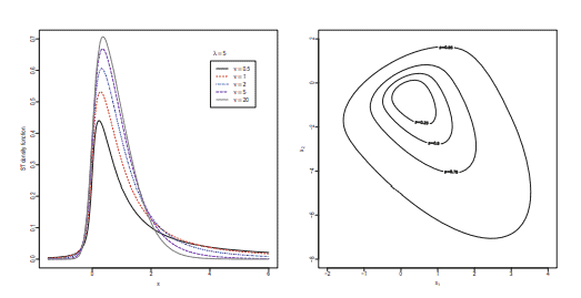
Some instances of density (1) are displayed in the left panel of Fig. 1. If $\lambda$ was replaced by $-\lambda$, the densities would be reflected on the opposite side of the vertical axis, since $-Y \sim \operatorname{ST}\left(-\xi, \omega^{2},-\lambda, \nu\right)$.
统计代写|生物统计代写biostatistics代考|Basic General Aspects
The high flexibility of the ST distribution makes it particularly appealing in a wide range of data fitting problems, more than its companion, the SN distribution. Reliable techniques for implementing connected MLE or other estimation methods are therefore crucial.
From the inference viewpoint, another advantage of the ST over the related SN distribution is the lack of a stationary point at $\lambda=0$ (or $\alpha=0$ in the multivariate case), and the implied singularity of the information matrix. This stationary point of the SN is systematic: it occurs for all samples, no matter what $n$ is. This peculiar aspect has been emphasized more than necessary in the literature, considering that it pertains to a single although important value of the parameter. Anyway, no such problem exists under the ST assumption. The lack of a stationary point at the origin was first observed empirically and welcomed as ‘a pleasant surprise’ by Azzalini and Capitanio (2003), but no theoretical explanation was given. Additional numerical evidence in this direction has been provided by Azzalini and Genton (2008). The theoretical explanation of why the SN and the ST likelihood functions behave differently was finally established by Hallin and Ley (2012).
Another peculiar aspect of the SN likelihood function is the possibility that the maximum of the likelihood function occurs at $\lambda=\pm \infty$, or at $|\alpha| \rightarrow \infty$ in the multivariate case. Note that this happens without divergence of the likelihood function, but only with divergence of the parameter achieving the maximum. In this respect the SN and the ST model are similar: both of them can lead to this pattern.
Differently from the stationarity point at the origin, the phenomenon of divergent estimates is transient: it occurs mostly with small $n$, and the probability of its occurrence decreases very rapidly when $n$ increases. However, when it occurs for the $n$ available data, we must handle it. There are different views among statisticians on whether such divergent values must be retained as valid estimates or they must be rejected as unacceptable. We embrace the latter view, for the reasons put forward by Azzalini and Arellano-Valle (2013), and adopt the maximum penalized likelihood estimate (MPLE) proposed there to prevent the problem. While the motivation for MPLE is primarily for small to moderate $n$, we use it throughout for consistency.
There is an additional peculiar feature of the ST log-likelihood function, which however we mention only for completeness, rather than for its real relevance. In cases when $v$ is allowed to span the whole positive half-line, poles of the likelihood function must exist near $v=0$, similarly to the case of a Student’s $t$ with unspecified degrees of freedom. This problem has been explored numerically by Azzalini and Capitanio (2003, pp. 384-385), and the indication was that these poles must exist at very small values of $v$, such as $\hat{v}=0.06$ in one specific instance.
This phenomenon is qualitatively similar to the problem of poles of the likelihood function for a finite mixture of continuous distributions. Even in the simple case of univariate normal components, there always exist $n$ poles on the boundary of the parameter space if the standard deviations of the components are unrestricted; see for instance Day (1969, Section 7). The problem is conceptually interesting, in both settings, but in practice it is easily dealt with in various ways. In the ST setting, the simplest solution is to impose a constraint $v>v_{0}>0$ where $v_{0}$ is some very small value, such as $v_{0}=0.1$ or $0.2$. Even if fitted to data, a $t$ or ST density with $v<0.1$ would be an object hard to use in practice.
生物统计代考
统计代写|生物统计代写biostatistics代考|Flexible Distributions: The Skew-t Case
在分布理论的背景下,一个中心主题是研究概率分布的灵活参数族,即当参数跨越其允许范围时,允许其行为发生实质性变化的族。
为简洁起见,我们将使用短语“灵活分布”来指代这个领域。该逻辑的原型构造由单变量连续变量的 Pearson 曲线系统表示。在这个公式中,密度函数由四个参数调节,允许偏度和峰度测量的广泛变化,因此提供比正态分布表示的基本情况更大的灵活性,其中只能调整位置和规模。
自 Pearson 时代以来,灵活分布一直是文献中持续关注的主题,近年来活动尤为激烈。新发展的一个显着特征是对多元分布的更多考虑,这反映了当前在更大数据集的应用工作中的可用性,无论是在样本大小还是维度上。在多变量设置中,各种公式通常具有四个参数块来调节位置、规模、偏度和峰度。
在为数据拟合提供强大工具的同时,当我们进入具体的估计阶段时,灵活的分布也带来了一些挑战。我们将使用最大似然估计 (MLE) 或其变体,但其他标准存在质量上类似的问题。估计的明确表达是不可能的;与拟合更简单的参数模型(例如 Gamma 或 Beta 分布)相比,总是涉及一些数值优化过程,并且由于涉及的参数数量较多,因此该过程并不是那么简单。此外,在某些情况下,这些参数族的灵活性可能会导致困难:如果数据模式没有稳定地指向参数空间的某个点,在对数似然或一些其他估计标准方面,可能有两个或更多这样的点构成相当有效的候选者。显然,这些问题在样本量较小的情况下更具挑战性,稍后表示n,因为对数似然函数(可能由先验分布调整)相对更平坦,但数值经验表明它们可以持续相当大n, 在某些情况下。
统计代写|生物统计代写biostatistics代考|The Skew-t Distribution: Basic Facts
在进入我们的实际开发之前,我们回顾一下关于连续分布的 ST 参数族的一些基本事实。在最简单的描述中,它是作为经典学生的扰动获得的吨分配。对于更具体的描述,从单变量设置开始,其中族的组件由四个参数标识。在这四个参数中,一个表示X在下文中规定了分配的位置;规模由正参数调节ω; 形状(代表背离对称)由λ; 尾重由在(和在>0),表示“自由度”,就像经典的吨分配。
在“标准情况”中引入分布很方便,即带有位置X=0和规模ω=1. 在这种情况下,密度函数是
吨(和;λ,在)=2吨(和;在)吨(λ和在+1在+和2;在+1),和∈R
在哪里
吨(和;在)=Γ(12(在+1))圆周率在Γ(12在)(1+和2在)−(在+1)/2,和∈R
是经典学生的密度函数吨上在自由度和吨(⋅;在)表示其分布函数;但是请注意,在(1)中,这是用在+1自由程度。另外,请注意符号吨用于 (1) 和 (2) 中的两个密度,它们的区别在于存在一个或两个参数。
如果从是具有密度函数 (1) 的随机变量,位置和尺度变换是=X+ω从有密度函数
吨是(X;θ)=ω−1吨(和;λ,在),和=ω−1(X−X),
在哪里θ=(X,ω,λ,在). 在这种情况下,我们写是∼英石(X,ω2,λ,在), 在哪里ω为与正态分布的通常表示法相似的平方。
什么时候λ=0,我们恢复由吨分布 (2)。什么时候在→∞,我们得到带有参数的偏正态(SN)分布(X,ω,λ),例如由 Azzalini 和 Capitanio(2014 年,第 2 章)描述。什么时候λ=0和在→∞, (3) 收敛到ñ(X,ω2)分配。
密度 (1) 的一些实例显示在图 1 的左侧面板中。如果λ被替换为−λ,密度将反映在垂直轴的另一侧,因为−是∼英石(−X,ω2,−λ,ν).
统计代写|生物统计代写biostatistics代考|Basic General Aspects
ST 分布的高度灵活性使其在广泛的数据拟合问题中特别有吸引力,超过了它的同伴 SN 分布。因此,实现互联 MLE 或其他估计方法的可靠技术至关重要。
从推理的角度来看,ST 相对于相关 SN 分布的另一个优势是在λ=0(或者一个=0在多变量情况下),以及信息矩阵的隐含奇异性。SN 的这个驻点是系统性的:它出现在所有样本中,无论如何n是。考虑到它与参数的单个但重要的值有关,在文献中已经过分强调了这一特殊方面。无论如何,在ST假设下不存在这样的问题。Azzalini 和 Capitanio(2003 年)首先凭经验观察到原点缺乏静止点,并称其为“惊喜”,但没有给出理论解释。Azzalini 和 Genton (2008) 提供了这方面的额外数字证据。Hallin 和 Ley (2012) 最终建立了关于 SN 和 ST 似然函数为何表现不同的理论解释。
SN 似然函数的另一个特殊方面是似然函数的最大值出现在λ=±∞, 或|一个|→∞在多变量情况下。请注意,这种情况在似然函数没有发散的情况下发生,但只有在参数的发散达到最大值的情况下才会发生。在这方面,SN 和 ST 模型是相似的:它们都可以导致这种模式。
与原点的平稳点不同,估计发散现象是短暂的:它主要发生在小n,并且它发生的概率在当n增加。然而,当它发生在n可用的数据,我们必须处理它。对于是否必须将这些不同的值保留为有效估计值还是必须将其视为不可接受的值而拒绝,统计学家之间存在不同的看法。由于 Azzalini 和 Arellano-Valle (2013) 提出的原因,我们接受后一种观点,并采用那里提出的最大惩罚似然估计 (MPLE) 来防止该问题。虽然 MPLE 的动机主要是针对中小型n,我们始终使用它以保持一致性。
ST 对数似然函数还有一个额外的特殊功能,但是我们仅出于完整性而不是其真正相关性而提及它。在某些情况下在允许跨越整个正半线,似然函数的极点必须存在于附近在=0,类似于学生的情况吨具有未指定的自由度。Azzalini 和 Capitanio (2003, pp. 384-385) 对这个问题进行了数值研究,表明这些极点必须以非常小的值存在在, 如在^=0.06在一个特定的情况下。
这种现象在性质上类似于连续分布的有限混合的似然函数极点问题。即使在单变量正态分量的简单情况下,也总是存在n如果分量的标准差不受限制,则参数空间边界上的极点;参见例如 Day (1969, Section 7)。在这两种情况下,这个问题在概念上都很有趣,但在实践中,它很容易以各种方式处理。在 ST 设置中,最简单的解决方案是施加约束在>在0>0在哪里在0是一些非常小的值,比如在0=0.1或者0.2. 即使适合数据,a吨或 ST 密度与在<0.1将是一个难以在实践中使用的对象。

统计代写请认准statistics-lab™. statistics-lab™为您的留学生涯保驾护航。
金融工程代写
金融工程是使用数学技术来解决金融问题。金融工程使用计算机科学、统计学、经济学和应用数学领域的工具和知识来解决当前的金融问题,以及设计新的和创新的金融产品。
非参数统计代写
非参数统计指的是一种统计方法,其中不假设数据来自于由少数参数决定的规定模型;这种模型的例子包括正态分布模型和线性回归模型。
广义线性模型代考
广义线性模型(GLM)归属统计学领域,是一种应用灵活的线性回归模型。该模型允许因变量的偏差分布有除了正态分布之外的其它分布。
术语 广义线性模型(GLM)通常是指给定连续和/或分类预测因素的连续响应变量的常规线性回归模型。它包括多元线性回归,以及方差分析和方差分析(仅含固定效应)。
有限元方法代写
有限元方法(FEM)是一种流行的方法,用于数值解决工程和数学建模中出现的微分方程。典型的问题领域包括结构分析、传热、流体流动、质量运输和电磁势等传统领域。
有限元是一种通用的数值方法,用于解决两个或三个空间变量的偏微分方程(即一些边界值问题)。为了解决一个问题,有限元将一个大系统细分为更小、更简单的部分,称为有限元。这是通过在空间维度上的特定空间离散化来实现的,它是通过构建对象的网格来实现的:用于求解的数值域,它有有限数量的点。边界值问题的有限元方法表述最终导致一个代数方程组。该方法在域上对未知函数进行逼近。[1] 然后将模拟这些有限元的简单方程组合成一个更大的方程系统,以模拟整个问题。然后,有限元通过变化微积分使相关的误差函数最小化来逼近一个解决方案。
tatistics-lab作为专业的留学生服务机构,多年来已为美国、英国、加拿大、澳洲等留学热门地的学生提供专业的学术服务,包括但不限于Essay代写,Assignment代写,Dissertation代写,Report代写,小组作业代写,Proposal代写,Paper代写,Presentation代写,计算机作业代写,论文修改和润色,网课代做,exam代考等等。写作范围涵盖高中,本科,研究生等海外留学全阶段,辐射金融,经济学,会计学,审计学,管理学等全球99%专业科目。写作团队既有专业英语母语作者,也有海外名校硕博留学生,每位写作老师都拥有过硬的语言能力,专业的学科背景和学术写作经验。我们承诺100%原创,100%专业,100%准时,100%满意。
随机分析代写
随机微积分是数学的一个分支,对随机过程进行操作。它允许为随机过程的积分定义一个关于随机过程的一致的积分理论。这个领域是由日本数学家伊藤清在第二次世界大战期间创建并开始的。
时间序列分析代写
随机过程,是依赖于参数的一组随机变量的全体,参数通常是时间。 随机变量是随机现象的数量表现,其时间序列是一组按照时间发生先后顺序进行排列的数据点序列。通常一组时间序列的时间间隔为一恒定值(如1秒,5分钟,12小时,7天,1年),因此时间序列可以作为离散时间数据进行分析处理。研究时间序列数据的意义在于现实中,往往需要研究某个事物其随时间发展变化的规律。这就需要通过研究该事物过去发展的历史记录,以得到其自身发展的规律。
回归分析代写
多元回归分析渐进(Multiple Regression Analysis Asymptotics)属于计量经济学领域,主要是一种数学上的统计分析方法,可以分析复杂情况下各影响因素的数学关系,在自然科学、社会和经济学等多个领域内应用广泛。
MATLAB代写
MATLAB 是一种用于技术计算的高性能语言。它将计算、可视化和编程集成在一个易于使用的环境中,其中问题和解决方案以熟悉的数学符号表示。典型用途包括:数学和计算算法开发建模、仿真和原型制作数据分析、探索和可视化科学和工程图形应用程序开发,包括图形用户界面构建MATLAB 是一个交互式系统,其基本数据元素是一个不需要维度的数组。这使您可以解决许多技术计算问题,尤其是那些具有矩阵和向量公式的问题,而只需用 C 或 Fortran 等标量非交互式语言编写程序所需的时间的一小部分。MATLAB 名称代表矩阵实验室。MATLAB 最初的编写目的是提供对由 LINPACK 和 EISPACK 项目开发的矩阵软件的轻松访问,这两个项目共同代表了矩阵计算软件的最新技术。MATLAB 经过多年的发展,得到了许多用户的投入。在大学环境中,它是数学、工程和科学入门和高级课程的标准教学工具。在工业领域,MATLAB 是高效研究、开发和分析的首选工具。MATLAB 具有一系列称为工具箱的特定于应用程序的解决方案。对于大多数 MATLAB 用户来说非常重要,工具箱允许您学习和应用专业技术。工具箱是 MATLAB 函数(M 文件)的综合集合,可扩展 MATLAB 环境以解决特定类别的问题。可用工具箱的领域包括信号处理、控制系统、神经网络、模糊逻辑、小波、仿真等。