如果你也在 怎样代写统计推断Statistical inference这个学科遇到相关的难题,请随时右上角联系我们的24/7代写客服。
统计推断是指从数据中得出关于种群或科学真理的结论的过程。进行推断的模式有很多,包括统计建模、面向数据的策略以及在分析中明确使用设计和随机化。
statistics-lab™ 为您的留学生涯保驾护航 在代写统计推断Statistical inference方面已经树立了自己的口碑, 保证靠谱, 高质且原创的统计Statistics代写服务。我们的专家在代写统计推断Statistical inference代写方面经验极为丰富,各种代写统计推断Statistical inference相关的作业也就用不着说。
我们提供的统计推断Statistical inference及其相关学科的代写,服务范围广, 其中包括但不限于:
- Statistical Inference 统计推断
- Statistical Computing 统计计算
- Advanced Probability Theory 高等概率论
- Advanced Mathematical Statistics 高等数理统计学
- (Generalized) Linear Models 广义线性模型
- Statistical Machine Learning 统计机器学习
- Longitudinal Data Analysis 纵向数据分析
- Foundations of Data Science 数据科学基础
统计代写|统计推断代写Statistical inference代考|Further exercises
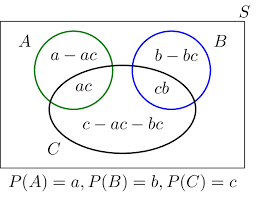
- Consider a probability space $(\Omega, \mathcal{F}, \mathrm{P})$ and events $A, B, C \in \mathcal{F}$.
(a) If $\mathrm{P}(A)=\frac{3}{4}$ and $\mathrm{P}(B)=\frac{1}{3}$, show that $\frac{1}{12} \leq \mathrm{P}(A \cap B) \leq \frac{1}{3}$. When do the two equalities hold?
(b) Is it possible to find events for which the following four conditions hold: $A \cap B \subset C^{c}, \mathrm{P}(A)>0.5, \mathrm{P}(B)>0.5$, and $\mathrm{P}(C)>0.5$ ?
(c) If $A \cap B \subset C^{c}, \mathrm{P}(A)=0.5$, and $\mathrm{P}(B)=0.5$, what is the largest possible value for $\mathrm{P}(C)$ ? - Consider a probability space $(\Omega, \mathcal{F}, \mathrm{P})$ and events $A, B, C \in \mathcal{F}$. Starting from the definition of probability measure, show that
(a) $\mathrm{P}\left((A \cup B) \cap\left(A^{c} \cup B^{c}\right)\right)=\mathrm{P}(A)+\mathrm{P}(B)-2 \mathrm{P}(A \cap B)$.
(b) $\mathrm{P}(A \cup B \cup C)=\mathrm{P}(A)+\mathrm{P}(B)+\mathrm{P}(C)-\mathrm{P}(A \cap B)-\mathrm{P}(A \cap C)-\mathrm{P}(B \cap C)+\mathrm{P}(A \cap B \cap C)$.
3.(a) In 1995 an account on the LSE network came with a three letter (all uppercase Roman letter) password. Suppose a malicious hacker could check one password every millisecond. Assuming the hacker knows a username and the format of passwords, what is the maximum time that it would take to break into an account?
(b) In a bid to improve security, IT services propose to either double the number of letters available (by including lowercase letters) or double the length (from three to six). Which of these options would you recommend? Is there a fundamental principle here that could be applied in other situations?
(c) Suppose that, to be on the safe side, IT services double the number of letters, include numbers, and increase the password length to twelve. You have forgotten your password. You remember that it contains the characters ${t, t, t, S, s, s, I, i, i, c, a, 3}$. If you can check passwords at the same rate as a hacker, how long will it take you to get into your account? - $A$ and $B$ are events of positive probability. Supply a proof for each of the following.
(a) If $A$ and $B$ are independent, $A$ and $B^{c}$ are independent.
(b) If $A$ and $B$ are independent, $\mathrm{P}\left(A^{c} \mid B^{c}\right)+\mathrm{P}(A \mid B)=1$.
(c) If $\mathrm{P}(A \mid B)<\mathrm{P}(A)$, then $\mathrm{P}(B \mid A)<\mathrm{P}(B)$.
(d) If $\mathrm{P}(B \mid A)=\mathrm{P}\left(B \mid A^{c}\right)$ then $A$ and $B$ are independent. - A fair coin is independently tossed twice. Consider the following events:
$A=$ “The first toss is heads”
$B=$ “The second toss is heads”
$C=$ “First and second toss show the same side”
Show that $A, B, C$ are pairwise independent events, but not independent events. - Show that, if $A, B$, and $C$ are independent events with $\mathrm{P}(A)=\mathrm{P}(B)=\mathrm{P}(C)$, then the probability that exactly one of $A, B$, and $C$ occurs is less than or equal to $4 / 9$.
- Consider a probability space $(\Omega, \mathcal{F}, \mathrm{P})$ and events $A, B, C_{1}, C_{2} \in \mathcal{F}$. Suppose, in addition, that $C_{1} \cap C_{2}=\varnothing$ and $C_{1} \cup C_{2}=B$. Show that
$$
\mathrm{P}(A \mid B)=\mathrm{P}\left(A \mid C_{1}\right) \mathrm{P}\left(C_{1} \mid B\right)+\mathrm{P}\left(A \mid C_{2}\right) \mathrm{P}\left(C_{2} \mid B\right) .
$$
统计代写|统计推断代写Statistical inference代考|Mapping outcomes to real numbers
At an intuitive level, the definition of a random variable is straightforward; a random variable is a quantity whose value is determined by the outcome of the experiment. The value taken by a random variable is always real. The randomness of a random variable is a consequence of our uncertainty about the outcome of the experiment. Example 3.1.1 illustrates this intuitive thinking, using the setup described in Example 2.4.14 as a starting point.
In practice, the quantities we model using random variables may be the output of systems that cannot be viewed as experiments in the strict sense. What these systems have in common, however, is that they are stochastic, rather than deterministic. This is an important distinction; for a deterministic system, if we know the input, we can determine exactly what the output will be. This is not true for a stochastic model, as its output is (at least in part) determined by a random element. We will encounter again the distinction between stochastic and deterministic systems in Chapter 12 , in the context of random-number generation.
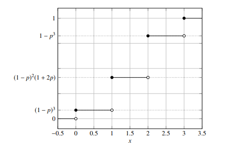
Example 3.1.1 (Coin flipping again)
Define a random variable $X$ to be the number of heads when we flip a coin three times. We assume that flips are independent and that the probability of a head at each flip is $p$. We know that $X$ can take one of four values, $0,1,2$, or 3 . For convenience,
we say that $X$ can take any real value, but the probability of it taking a value outside ${0,1,2,3}$ is zero. The probabilities evaluated in Example 2.4.14 can now be written as
$$
P(X=x)= \begin{cases}(1-p)^{3}, & x=0 \ 3 p(1-p)^{2}, & x=1 \ 3 p^{2}(1-p), & x=2 \ p^{3}, & x=3 \ 0, & \text { otherwise }\end{cases}
$$
统计代写|统计推断代写Statistical inference代考|Cumulative distribution functions
As mentioned above, we are usually more interested in probabilities associated with a random variable than in a mapping from outcomes to real numbers. The probability associated with a random variable is completely characterised by its cumulative distribution function.
Definition 3.2.1 (Cumulative distribution function)
The cumulative distribution function (CDF) of a random variable $X$ is the function $F_{X}: \mathbb{R} \longrightarrow[0,1]$ given by $F_{X}(x)=\mathrm{P}(X \leq x)$
A couple of points to note about cumulative distribution functions.
- We will use $F_{X}$ to denote the cumulative distribution function of the random variable $X, F_{Y}$ to denote the cumulative distribution function of the random variable $Y$, and so on.
- Be warned; some texts use the argument to identify different distribution functions. For example, you may see $F(x)$ and $F(y)$ used, not to denote the same function applied to different arguments, but to indicate a value of the cumulative distribution function of $X$ and a value of the cumulative distribution function of $Y$. This can be deeply confusing and we will try to avoid doing it.
In our discussion of the properties of cumulative distribution functions, the following definition is useful.
Definition 3.2.2 (Right continuity)
A function $g: \mathbb{R} \rightarrow \mathbb{R}$ is right-continuous if $g(x+)=g(x)$ for all $x \in \mathbb{R}$, where $g(x+)=\lim _{h \downarrow 0} g(x+h)$
The notation $g(x+)$ is used for limit from the right. There is nothing complicated about this; it is just the limit of the values given by $g$ as we approach the point $x$ from the right-hand side. Right continuity says that we can approach any point from the right-hand side without encountering a jump in the value given by $g$. There is an analogous definition of left continuity in terms of the limit from the left; $g$ is left-continuous if $g(x-)=\lim {h \downarrow 0} g(x-h)=g(x)$ for all $x$. Somewhat confusingly, the notation $\lim {h \uparrow 0}$ is sometimes used. This is discussed as part of Exercise 3.2.
The elementary properties of cumulative distribution functions are inherited from their definition in terms of probability. It is true, but rather harder to show, that any function satisfying the three properties given in Proposition $3.2 .3$ is the distribution function of some random variable. We will only prove necessity of the three conditions.
统计推断代考
统计代写|统计推断代写Statistical inference代考|Further exercises
- 考虑一个概率空间(Ω,F,磷)和事件一个,乙,C∈F.
(a) 如果磷(一个)=34和磷(乙)=13, 显示112≤磷(一个∩乙)≤13. 这两个等式何时成立?
(b) 是否有可能找到满足以下四个条件的事件:一个∩乙⊂CC,磷(一个)>0.5,磷(乙)>0.5, 和磷(C)>0.5?
(c) 如果一个∩乙⊂CC,磷(一个)=0.5, 和磷(乙)=0.5, 的最大可能值是多少磷(C) ? - 考虑一个概率空间(Ω,F,磷)和事件一个,乙,C∈F. 从概率测度的定义出发,证明
(a)磷((一个∪乙)∩(一个C∪乙C))=磷(一个)+磷(乙)−2磷(一个∩乙).
(二)磷(一个∪乙∪C)=磷(一个)+磷(乙)+磷(C)−磷(一个∩乙)−磷(一个∩C)−磷(乙∩C)+磷(一个∩乙∩C).
3.(a) 1995 年,LSE 网络上的一个帐户带有三个字母(全为大写罗马字母)的密码。假设恶意黑客可以每毫秒检查一个密码。假设黑客知道用户名和密码格式,那么入侵帐户所需的最长时间是多少?
(b) 为了提高安全性,IT 服务建议将可用字母的数量增加一倍(包括小写字母)或将长度增加一倍(从 3 个到 6 个)。您会推荐以下哪些选项?这里有一个基本原则可以应用于其他情况吗?
(c) 假设为了安全起见,IT 服务将字母数量加倍,包括数字,并将密码长度增加到 12。您忘记了密码。你记得它包含字符吨,吨,吨,小号,s,s,我,一世,一世,C,一个,3. 如果您可以像黑客一样检查密码,您需要多长时间才能进入您的帐户? - 一个和乙是正概率事件。为以下每一项提供证明。
(a) 如果一个和乙是独立的,一个和乙C是独立的。
(b) 如果一个和乙是独立的,磷(一个C∣乙C)+磷(一个∣乙)=1.
(c) 如果磷(一个∣乙)<磷(一个), 然后磷(乙∣一个)<磷(乙).
(d) 如果磷(乙∣一个)=磷(乙∣一个C)然后一个和乙是独立的。 - 一枚公平的硬币独立投掷两次。考虑以下事件:
一个=“第一次投掷是正面”
乙=“第二次投掷是正面”
C=“第一次和第二次折腾显示同一面”
表明一个,乙,C是成对独立事件,但不是独立事件。 - 证明,如果一个,乙, 和C是独立的事件磷(一个)=磷(乙)=磷(C),那么恰好其中之一的概率一个,乙, 和C发生小于或等于4/9.
- 考虑一个概率空间(Ω,F,磷)和事件一个,乙,C1,C2∈F. 此外,假设C1∩C2=∅和C1∪C2=乙. 显示
磷(一个∣乙)=磷(一个∣C1)磷(C1∣乙)+磷(一个∣C2)磷(C2∣乙).
统计代写|统计推断代写Statistical inference代考|Mapping outcomes to real numbers
在直观的层面上,随机变量的定义很简单;随机变量是一个量,其值由实验结果决定。随机变量取的值总是实数。随机变量的随机性是我们对实验结果的不确定性的结果。示例 3.1.1 说明了这种直观的想法,使用示例 2.4.14 中描述的设置作为起点。
在实践中,我们使用随机变量建模的数量可能是系统的输出,不能被视为严格意义上的实验。然而,这些系统的共同点是它们是随机的,而不是确定的。这是一个重要的区别; 对于确定性系统,如果我们知道输入,我们就可以准确地确定输出将是什么。对于随机模型而言,情况并非如此,因为其输出(至少部分)由随机元素确定。在第 12 章中,我们将在随机数生成的背景下再次遇到随机系统和确定性系统之间的区别。
示例 3.1.1(再次抛硬币)
定义一个随机变量X是我们掷硬币 3 次时正面朝上的次数。我们假设翻转是独立的,并且每次翻转出现正面的概率是p. 我们知道X可以取四个值之一,0,1,2,或 3 。为了方便,
我们说X可以取任何实际值,但它取值的概率在外面0,1,2,3为零。示例 2.4.14 中评估的概率现在可以写为
磷(X=X)={(1−p)3,X=0 3p(1−p)2,X=1 3p2(1−p),X=2 p3,X=3 0, 否则
统计代写|统计推断代写Statistical inference代考|Cumulative distribution functions
如上所述,我们通常对与随机变量相关的概率比对从结果到实数的映射更感兴趣。与随机变量相关的概率完全由它的累积分布函数来表征。
定义 3.2.1(累积分布函数)
随机变量的累积分布函数(CDF)X是函数FX:R⟶[0,1]由FX(X)=磷(X≤X)
关于累积分布函数需要注意的几点。
- 我们将使用FX表示随机变量的累积分布函数X,F是表示随机变量的累积分布函数是, 等等。
- 被警告; 一些文本使用参数来识别不同的分布函数。例如,您可能会看到F(X)和F(是)使用,不是表示应用于不同参数的相同函数,而是表示累积分布函数的值X和累积分布函数的值是. 这可能会让人非常困惑,我们会尽量避免这样做。
在我们讨论累积分布函数的性质时,以下定义很有用。
定义 3.2.2(右连续性)
函数G:R→R是右连续的,如果G(X+)=G(X)对所有人X∈R, 在哪里G(X+)=林H↓0G(X+H)
符号G(X+)用于从右侧限制。这没有什么复杂的。这只是给出的值的限制G当我们接近重点时X从右侧。右连续性表示我们可以从右侧接近任何点,而不会遇到下式给出的值的跳跃G. 就左极限而言,左连续性有一个类似的定义;G是左连续的,如果G(X−)=林H↓0G(X−H)=G(X)对所有人X. 有点令人困惑的是,符号林H↑0有时使用。这将作为练习 3.2 的一部分进行讨论。
累积分布函数的基本性质是从它们在概率方面的定义中继承而来的。确实,但更难证明,任何满足命题中给出的三个属性的函数3.2.3是某个随机变量的分布函数。我们只会证明这三个条件的必要性。

统计代写请认准statistics-lab™. statistics-lab™为您的留学生涯保驾护航。
金融工程代写
金融工程是使用数学技术来解决金融问题。金融工程使用计算机科学、统计学、经济学和应用数学领域的工具和知识来解决当前的金融问题,以及设计新的和创新的金融产品。
非参数统计代写
非参数统计指的是一种统计方法,其中不假设数据来自于由少数参数决定的规定模型;这种模型的例子包括正态分布模型和线性回归模型。
广义线性模型代考
广义线性模型(GLM)归属统计学领域,是一种应用灵活的线性回归模型。该模型允许因变量的偏差分布有除了正态分布之外的其它分布。
术语 广义线性模型(GLM)通常是指给定连续和/或分类预测因素的连续响应变量的常规线性回归模型。它包括多元线性回归,以及方差分析和方差分析(仅含固定效应)。
有限元方法代写
有限元方法(FEM)是一种流行的方法,用于数值解决工程和数学建模中出现的微分方程。典型的问题领域包括结构分析、传热、流体流动、质量运输和电磁势等传统领域。
有限元是一种通用的数值方法,用于解决两个或三个空间变量的偏微分方程(即一些边界值问题)。为了解决一个问题,有限元将一个大系统细分为更小、更简单的部分,称为有限元。这是通过在空间维度上的特定空间离散化来实现的,它是通过构建对象的网格来实现的:用于求解的数值域,它有有限数量的点。边界值问题的有限元方法表述最终导致一个代数方程组。该方法在域上对未知函数进行逼近。[1] 然后将模拟这些有限元的简单方程组合成一个更大的方程系统,以模拟整个问题。然后,有限元通过变化微积分使相关的误差函数最小化来逼近一个解决方案。
tatistics-lab作为专业的留学生服务机构,多年来已为美国、英国、加拿大、澳洲等留学热门地的学生提供专业的学术服务,包括但不限于Essay代写,Assignment代写,Dissertation代写,Report代写,小组作业代写,Proposal代写,Paper代写,Presentation代写,计算机作业代写,论文修改和润色,网课代做,exam代考等等。写作范围涵盖高中,本科,研究生等海外留学全阶段,辐射金融,经济学,会计学,审计学,管理学等全球99%专业科目。写作团队既有专业英语母语作者,也有海外名校硕博留学生,每位写作老师都拥有过硬的语言能力,专业的学科背景和学术写作经验。我们承诺100%原创,100%专业,100%准时,100%满意。
随机分析代写
随机微积分是数学的一个分支,对随机过程进行操作。它允许为随机过程的积分定义一个关于随机过程的一致的积分理论。这个领域是由日本数学家伊藤清在第二次世界大战期间创建并开始的。
时间序列分析代写
随机过程,是依赖于参数的一组随机变量的全体,参数通常是时间。 随机变量是随机现象的数量表现,其时间序列是一组按照时间发生先后顺序进行排列的数据点序列。通常一组时间序列的时间间隔为一恒定值(如1秒,5分钟,12小时,7天,1年),因此时间序列可以作为离散时间数据进行分析处理。研究时间序列数据的意义在于现实中,往往需要研究某个事物其随时间发展变化的规律。这就需要通过研究该事物过去发展的历史记录,以得到其自身发展的规律。
回归分析代写
多元回归分析渐进(Multiple Regression Analysis Asymptotics)属于计量经济学领域,主要是一种数学上的统计分析方法,可以分析复杂情况下各影响因素的数学关系,在自然科学、社会和经济学等多个领域内应用广泛。
MATLAB代写
MATLAB 是一种用于技术计算的高性能语言。它将计算、可视化和编程集成在一个易于使用的环境中,其中问题和解决方案以熟悉的数学符号表示。典型用途包括:数学和计算算法开发建模、仿真和原型制作数据分析、探索和可视化科学和工程图形应用程序开发,包括图形用户界面构建MATLAB 是一个交互式系统,其基本数据元素是一个不需要维度的数组。这使您可以解决许多技术计算问题,尤其是那些具有矩阵和向量公式的问题,而只需用 C 或 Fortran 等标量非交互式语言编写程序所需的时间的一小部分。MATLAB 名称代表矩阵实验室。MATLAB 最初的编写目的是提供对由 LINPACK 和 EISPACK 项目开发的矩阵软件的轻松访问,这两个项目共同代表了矩阵计算软件的最新技术。MATLAB 经过多年的发展,得到了许多用户的投入。在大学环境中,它是数学、工程和科学入门和高级课程的标准教学工具。在工业领域,MATLAB 是高效研究、开发和分析的首选工具。MATLAB 具有一系列称为工具箱的特定于应用程序的解决方案。对于大多数 MATLAB 用户来说非常重要,工具箱允许您学习和应用专业技术。工具箱是 MATLAB 函数(M 文件)的综合集合,可扩展 MATLAB 环境以解决特定类别的问题。可用工具箱的领域包括信号处理、控制系统、神经网络、模糊逻辑、小波、仿真等。