如果你也在 怎样代写统计推断statistics interference这个学科遇到相关的难题,请随时右上角联系我们的24/7代写客服。
统计推断是利用数据分析来推断概率基础分布的属性的过程。 推断性统计分析推断人口的属性,例如通过测试假设和得出估计值。
statistics-lab™ 为您的留学生涯保驾护航 在代写统计推断statistics interference方面已经树立了自己的口碑, 保证靠谱, 高质且原创的统计Statistics代写服务。我们的专家在代写统计推断statistics interference方面经验极为丰富,各种代写统计推断statistics interference相关的作业也就用不着说。
我们提供的属性统计推断statistics interference及其相关学科的代写,服务范围广, 其中包括但不限于:
- Statistical Inference 统计推断
- Statistical Computing 统计计算
- Advanced Probability Theory 高等楖率论
- Advanced Mathematical Statistics 高等数理统计学
- (Generalized) Linear Models 广义线性模型
- Statistical Machine Learning 统计机器学习
- Longitudinal Data Analysis 纵向数据分析
- Foundations of Data Science 数据科学基础
统计代写|统计推断作业代写statistics interference代考|Relation with acceptance and rejection
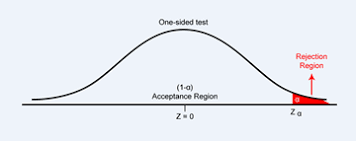
There is a conceptual difference, but essentially no mathematical difference, between the discussion here and the treatment of testing as a two-decision problem, with control over the formal error probabilities. In this we fix in principle the probability of rejecting $H_{0}$ when it is true, usually denoted by $\alpha$, aiming to maximize the probability of rejecting $H_{0}$ when false. This approach demands the explicit formulation of alternative possibilities. Essentially it amounts to setting in advance a threshold for $p_{o b s}$. It is, of course, potentially appropriate when clear decisions are to be made, as for example in some classification problems. The previous discussion seems to match more closely scientific practice in these matters, at least for those situations where analysis and interpretation rather than decision-making are the focus.
That is, there is a distinction between the Neyman-Pearson formulation of testing regarded as clarifying the meaning of statistical significance via hypothetical repetitions and that same theory regarded as in effect an instruction on how to implement the ideas by choosing a suitable $\alpha$ in advance and reaching different decisions accordingly. The interpretation to be attached to accepting or rejecting a hypothesis is strongly context-dependent; the point at stake here, however, is more a question of the distinction between assessing evidence, as contrasted with deciding by a formal rule which of two directions to take.
统计代写|统计推断作业代写statistics interference代考|Formulation of alternatives and test statistics
As set out above, the simplest version of a significance test involves formulation of a null hypothesis $H_{0}$ and a test statistic $T$, large, or possibly extreme, values of which point against $H_{0}$. Choice of $T$ is crucial in specifying the kinds of departure from $H_{0}$ of concern. In this first formulation no alternative probability models are explicitly formulated; an implicit family of possibilities is
specified via $T$. In fact many quite widely used statistical tests were developed in this way.
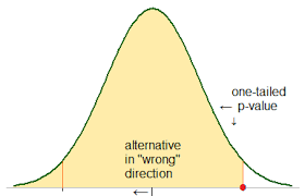
A second possibility is that the null hypothesis corresponds to a particular parameter value, say $\psi=\psi_{0}$, in a family of models and the departures of main interest correspond either, in the one-dimensional case, to one-sided alternatives $\psi>\psi_{0}$ or, more generally, to alternatives $\psi \neq \psi_{0}$. This formulation will suggest the most sensitive test statistic, essentially equivalent to the best estimate of $\psi$, and in the Neyman-Pearson formulation such an explicit formulation of alternatives is essential.
The approaches are, however, not quite as disparate as they may seem. Let $f_{0}(y)$ denote the density of the observations under $H_{0}$. Then we may associate with a proposed test statistic $T$ the exponential family
$$
f_{0}(y) \exp {t \theta-k(\theta)}
$$
where $k(\theta)$ is a normalizing constant. Then the test of $\theta=0$ most sensitive to these departures is based on $T$. Not all useful tests appear natural when viewed in this way, however; see, for instance, Example 3.5.
Many of the test procedures for examining model adequacy that are provided in standard software are best regarded as defined directly by the test statistic used rather than by a family of alternatives. In principle, as emphasized above, the null hypothesis is the conditional distribution of the data given the sufficient statistic for the parameters in the model. Then, within that null distribution, interesting directions of departure are identified.
The important distinction is between situations in which a whole family of distributions arises naturally as a base for analysis versus those where analysis is at a stage where only the null hypothesis is of explicit interest.
Tests where the null hypotheses itself is formulated in terms of arbitrary distributions, so-called nonparametric or distribution-free tests, illustrate the use of test statistics that are formulated largely or wholly informally, without specific probabilistically formulated alternatives in mind. To illustrate the arguments involved, consider initially a single homogenous set of observations.
统计代写|统计推断作业代写statistics interference代考|Relation with interval estimation
While conceptually it may seem simplest to regard estimation with uncertainty as a simpler and more direct mode of analysis than significance testing there are some important advantages, especially in dealing with relatively complicated problems, in arguing in the other direction. Essentially confidence intervals, or more generally confidence sets, can be produced by testing consistency with every possible value in $\Omega_{\psi}$ and taking all those values not ‘rejected’ at level $c$, say, to produce a $1-c$ level interval or region. This procedure has the property that in repeated applications any true value of $\psi$ will be included in the region except in a proportion $1-c$ of cases. This can be done at various levels $c$, using the same form of test throughout.
Example 3.6. Ratio of normal means. Given two independent sets of random variables from normal distributions of unknown means $\mu_{0}, \mu_{1}$ and with known variance $\sigma_{0}^{2}$, we first reduce by sufficiency to the sample means $\bar{y}{0}, \bar{y}{1}$. Suppose that the parameter of interest is $\psi=\mu_{1} / \mu_{0}$. Consider the null hypothesis $\psi=\psi_{0}$. Then we look for a statistic with a distribution under the null hypothesis that does not depend on the nuisance parameter. Such a statistic is
$$
\frac{\bar{Y}{1}-\psi{0} \bar{Y}{0}}{\sigma{0} \sqrt{\left(1 / n_{1}+\psi_{0}^{2} / n_{0}\right)}}
$$
this has a standard normal distribution under the null hypothesis. This with $\psi_{0}$ replaced by $\psi$ could be treated as a pivot provided that we can treat $\bar{Y}_{0}$ as positive.
Note that provided the two distributions have the same variance a similar result with the Student $t$ distribution replacing the standard normal would apply if the variance were unknown and had to be estimated. To treat the probably more realistic situation where the two distributions have different and unknown variances requires the approximate techniques of Chapter $6 .$
We now form a $1-c$ level confidence region by taking all those values of $\psi_{0}$ that would not be ‘rejected’ at level $c$ in this test. That is, we take the set
$$
\left{\psi: \frac{\left(\bar{Y}{1}-\psi \bar{Y}{0}\right)^{2}}{\sigma_{0}^{2}\left(1 / n_{1}+\psi^{2} / n_{0}\right)} \leq k_{1 ; c}^{}\right}, $$ where $k_{1 ; c}^{}$ is the upper $c$ point of the chi-squared distribution with one degree of freedom.
Thus we find the limits for $\psi$ as the roots of a quadratic equation. If there are no real roots, all values of $\psi$ are consistent with the data at the level in question. If the numerator and especially the denominator are poorly determined, a confidence interval consisting of the whole line may be the only rational conclusion to be drawn and is entirely reasonable from a testing point of view, even though regarded from a confidence interval perspective it may, wrongly, seem like a vacuous statement.
属性数据分析
统计代写|统计推断作业代写statistics interference代考|Relation with acceptance and rejection
此处的讨论与将测试视为两个决策问题并控制形式错误概率之间存在概念差异,但本质上没有数学差异。在此,我们原则上修复了在 $H_{0}$ 为真时拒绝的概率,通常用 $\alpha$ 表示,旨在最大化在错误时拒绝 $H_{0}$ 的概率。这种方法需要明确表述替代的可能性。本质上,它相当于为 $p_{obs}$ 预先设置了一个阈值。当然,当要做出明确的决定时,它可能是合适的,例如在一些分类问题中。之前的讨论似乎更符合这些问题的科学实践,
也就是说,Neyman-Pearson 的检验公式被认为是通过假设重复来阐明统计显着性的含义,而同一理论实际上被认为是关于如何通过选择合适的 $\alpha$ 来实施这些想法的指导。提前并相应地做出不同的决定。接受或拒绝假设的解释强烈依赖于上下文;然而,这里的关键点更多地是评估证据之间的区别问题,与通过正式规则决定采取两个方向中的哪一个形成对比。
统计代写|统计推断作业代写statistics interference代考|Formulation of alternatives and test statistics
如上所述,显着性检验的最简单版本涉及制定原假设 $H_{0}$ 和检验统计量 $T$,其值相对于 $H_{0}$ 较大或可能极端。$T$ 的选择对于指定偏离关注的 $H_{0}$ 的种类至关重要。在第一个公式中,没有明确公式化替代概率模型;一个隐含的可能性族是
通过 $T$ 指定。事实上,许多相当广泛使用的统计测试都是以这种方式开发的。
第二种可能性是,原假设对应于模型族中的特定参数值,例如 $\psi=\psi_{0}$,并且主要兴趣的偏离在一维情况下对应于一个边替代$\psi>\psi_{0}$,或者更一般地说,替代$\psi \neq \psi_{0}$。这个公式将建议最敏感的测试统计量,基本上等同于 $\psi$ 的最佳估计,并且在 Neyman-Pearson 公式中,这样一个明确的替代公式是必不可少的。
然而,这些方法并不像看起来那样完全不同。令 $f_{0}(y)$ 表示 $H_{0}$ 下的观测密度。然后我们可以将一个建议的检验统计量 $T$ 与指数族
$$
f_{0}(y) \exp {t \theta-k(\theta)}
$$相关联
,其中 $k(\theta)$ 是归一化的持续的。那么对这些偏离最敏感的$\theta=0$ 的检验是基于$T$。然而,当以这种方式查看时,并非所有有用的测试都显得自然。例如,参见示例 3.5。
标准软件中提供的用于检查模型充分性的许多测试程序最好被视为由所使用的测试统计量直接定义,而不是由一系列替代方案定义。原则上,如上所述,零假设是给定模型中参数的充分统计数据的条件分布。然后,在该零分布中,识别出有趣的出发方向。
重要的区别在于整个分布家族作为分析基础自然出现的情况与分析处于只有零假设明确感兴趣的阶段的情况之间的区别。
零假设本身是根据任意分布制定的检验,即所谓的非参数或无分布检验,说明了在很大程度上或完全非正式地制定的检验统计量的使用,而没有考虑到特定的概率制定的替代方案。为了说明所涉及的论点,首先考虑一组同质的观察。
统计代写|统计推断作业代写statistics interference代考|Relation with interval estimation
虽然从概念上讲,将不确定性估计视为比显着性检验更简单和更直接的分析模式似乎最简单,但在另一个方向争论时,有一些重要的优势,特别是在处理相对复杂的问题时。本质上,置信区间,或更一般的置信集,可以通过测试 $\Omega_{\psi}$ 中每个可能值的一致性并取所有在 $c$ 级别未被“拒绝”的值来生成,例如,生成 $1 -c$ 级别区间或区域。这个过程的特性是在重复应用中,任何 $\psi$ 的真值都将包含在该区域中,但比例为 $1-c$ 的情况除外。这可以在各个级别 $c$ 上完成,始终使用相同的测试形式。
例 3.6。正常均值的比率。给定来自未知均值 $\mu_{0}、\mu_{1}$ 和已知方差 $\sigma_{0}^{2}$ 的正态分布的两组独立随机变量,我们首先通过充分性减少样本表示 $\bar{y} {0},\bar{y} {1}$。假设感兴趣的参数是 $\psi=\mu_{1} / \mu_{0}$。考虑原假设 $\psi=\psi_{0}$。然后我们在不依赖于讨厌参数的原假设下寻找具有分布的统计量。这样的统计量是
$$
\frac{\bar{Y}{1}-\psi{0} \bar{Y}{0}}{\sigma{0} \sqrt{\left(1 / n_{1} +\psi_{0}^{2} / n_{0}\right)}}
$$
这在原假设下具有标准正态分布。如果我们可以将 $\bar{Y}_{0}$ 视为正数,则将 $\psi_{0}$ 替换为 $\psi$ 可以被视为枢轴。
请注意,如果这两个分布具有相同的方差,则如果方差未知且必须估计,则使用 Student $t$ 分布替换标准正态的类似结果将适用。要处理可能更现实的情况,即两个分布具有不同且未知的方差,需要使用第 6 章的近似技术。
我们现在通过获取在此测试中不会在 $c$ 级别“拒绝”的所有 $\psi_{0}$ 值来形成 $1-c$ 级别的置信区域。也就是说,我们取集合
$$
\left{\psi: \frac{\left(\bar{Y}{1}-\psi \bar{Y}{0}\right)^{2}}{\ sigma_{0}^{2}\left(1 / n_{1}+\psi^{2} / n_{0}\right)} \leq k_{1 ; c}^{}\right}, $$ 其中 $k_{1 ; c}^{}$ 是具有一个自由度的卡方分布的上 $c$ 点。
因此,我们发现 $\psi$ 的极限是二次方程的根。如果没有实根,$\psi$ 的所有值都与相关级别的数据一致。如果分子,尤其是分母确定得不好,则由整条线组成的置信区间可能是唯一要得出的合理结论,并且从测试的角度来看是完全合理的,即使从置信区间的角度来看它可能,错误地,似乎是一个空洞的陈述。

统计代写请认准statistics-lab™. statistics-lab™为您的留学生涯保驾护航。统计代写|python代写代考
随机过程代考
在概率论概念中,随机过程是随机变量的集合。 若一随机系统的样本点是随机函数,则称此函数为样本函数,这一随机系统全部样本函数的集合是一个随机过程。 实际应用中,样本函数的一般定义在时间域或者空间域。 随机过程的实例如股票和汇率的波动、语音信号、视频信号、体温的变化,随机运动如布朗运动、随机徘徊等等。
贝叶斯方法代考
贝叶斯统计概念及数据分析表示使用概率陈述回答有关未知参数的研究问题以及统计范式。后验分布包括关于参数的先验分布,和基于观测数据提供关于参数的信息似然模型。根据选择的先验分布和似然模型,后验分布可以解析或近似,例如,马尔科夫链蒙特卡罗 (MCMC) 方法之一。贝叶斯统计概念及数据分析使用后验分布来形成模型参数的各种摘要,包括点估计,如后验平均值、中位数、百分位数和称为可信区间的区间估计。此外,所有关于模型参数的统计检验都可以表示为基于估计后验分布的概率报表。
广义线性模型代考
广义线性模型(GLM)归属统计学领域,是一种应用灵活的线性回归模型。该模型允许因变量的偏差分布有除了正态分布之外的其它分布。
statistics-lab作为专业的留学生服务机构,多年来已为美国、英国、加拿大、澳洲等留学热门地的学生提供专业的学术服务,包括但不限于Essay代写,Assignment代写,Dissertation代写,Report代写,小组作业代写,Proposal代写,Paper代写,Presentation代写,计算机作业代写,论文修改和润色,网课代做,exam代考等等。写作范围涵盖高中,本科,研究生等海外留学全阶段,辐射金融,经济学,会计学,审计学,管理学等全球99%专业科目。写作团队既有专业英语母语作者,也有海外名校硕博留学生,每位写作老师都拥有过硬的语言能力,专业的学科背景和学术写作经验。我们承诺100%原创,100%专业,100%准时,100%满意。
机器学习代写
随着AI的大潮到来,Machine Learning逐渐成为一个新的学习热点。同时与传统CS相比,Machine Learning在其他领域也有着广泛的应用,因此这门学科成为不仅折磨CS专业同学的“小恶魔”,也是折磨生物、化学、统计等其他学科留学生的“大魔王”。学习Machine learning的一大绊脚石在于使用语言众多,跨学科范围广,所以学习起来尤其困难。但是不管你在学习Machine Learning时遇到任何难题,StudyGate专业导师团队都能为你轻松解决。
多元统计分析代考
基础数据: $N$ 个样本, $P$ 个变量数的单样本,组成的横列的数据表
变量定性: 分类和顺序;变量定量:数值
数学公式的角度分为: 因变量与自变量
时间序列分析代写
随机过程,是依赖于参数的一组随机变量的全体,参数通常是时间。 随机变量是随机现象的数量表现,其时间序列是一组按照时间发生先后顺序进行排列的数据点序列。通常一组时间序列的时间间隔为一恒定值(如1秒,5分钟,12小时,7天,1年),因此时间序列可以作为离散时间数据进行分析处理。研究时间序列数据的意义在于现实中,往往需要研究某个事物其随时间发展变化的规律。这就需要通过研究该事物过去发展的历史记录,以得到其自身发展的规律。
回归分析代写
多元回归分析渐进(Multiple Regression Analysis Asymptotics)属于计量经济学领域,主要是一种数学上的统计分析方法,可以分析复杂情况下各影响因素的数学关系,在自然科学、社会和经济学等多个领域内应用广泛。
MATLAB代写
MATLAB 是一种用于技术计算的高性能语言。它将计算、可视化和编程集成在一个易于使用的环境中,其中问题和解决方案以熟悉的数学符号表示。典型用途包括:数学和计算算法开发建模、仿真和原型制作数据分析、探索和可视化科学和工程图形应用程序开发,包括图形用户界面构建MATLAB 是一个交互式系统,其基本数据元素是一个不需要维度的数组。这使您可以解决许多技术计算问题,尤其是那些具有矩阵和向量公式的问题,而只需用 C 或 Fortran 等标量非交互式语言编写程序所需的时间的一小部分。MATLAB 名称代表矩阵实验室。MATLAB 最初的编写目的是提供对由 LINPACK 和 EISPACK 项目开发的矩阵软件的轻松访问,这两个项目共同代表了矩阵计算软件的最新技术。MATLAB 经过多年的发展,得到了许多用户的投入。在大学环境中,它是数学、工程和科学入门和高级课程的标准教学工具。在工业领域,MATLAB 是高效研究、开发和分析的首选工具。MATLAB 具有一系列称为工具箱的特定于应用程序的解决方案。对于大多数 MATLAB 用户来说非常重要,工具箱允许您学习和应用专业技术。工具箱是 MATLAB 函数(M 文件)的综合集合,可扩展 MATLAB 环境以解决特定类别的问题。可用工具箱的领域包括信号处理、控制系统、神经网络、模糊逻辑、小波、仿真等。