如果你也在 怎样代写贝叶斯分析Bayesian Analysis这个学科遇到相关的难题,请随时右上角联系我们的24/7代写客服。
贝叶斯分析,一种统计推断方法(以英国数学家托马斯-贝叶斯命名),允许人们将关于人口参数的先验信息与样本所含信息的证据相结合,以指导统计推断过程。
statistics-lab™ 为您的留学生涯保驾护航 在代写贝叶斯分析Bayesian Analysis方面已经树立了自己的口碑, 保证靠谱, 高质且原创的统计Statistics代写服务。我们的专家在代写贝叶斯分析Bayesian Analysis代写方面经验极为丰富,各种代写贝叶斯分析Bayesian Analysis相关的作业也就用不着说。
我们提供的贝叶斯分析Bayesian Analysis及其相关学科的代写,服务范围广, 其中包括但不限于:
- Statistical Inference 统计推断
- Statistical Computing 统计计算
- Advanced Probability Theory 高等概率论
- Advanced Mathematical Statistics 高等数理统计学
- (Generalized) Linear Models 广义线性模型
- Statistical Machine Learning 统计机器学习
- Longitudinal Data Analysis 纵向数据分析
- Foundations of Data Science 数据科学基础
统计代写|贝叶斯分析代写Bayesian Analysis代考|Bayes’ rule
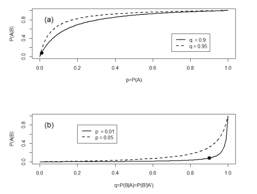
The starting point for Bayesian inference is Bayes’ rule. The simplest form of this is
$$
P(A \mid B)=\frac{P(A) P(B \mid A)}{P(A) P(B \mid A)+P(\bar{A}) P(B \mid \bar{A})},
$$
where $A$ and $B$ are events such that $P(B)>0$. This is easily proven by considering that:
$P(A \mid B)=\frac{P(A B)}{P(B)}$ by the definition of conditional probability $P(A B)=P(A) P(B \mid A) \quad$ by the multiplicative law of probability $P(B)=P(A B)+P(\bar{A} B)=P(A) P(B \mid A)+P(\bar{A}) P(B \mid \bar{A})$
by the law of total probability.
We see that the posterior probability $P(A \mid B)$ is equal to the prior probability $P(A)$ multiplied by a factor, where this factor is given by $P(B \mid A) / P(B)$
As regards terminology, we call $P(A)$ the prior probability of $A$ (meaning the probability of $A$ before $B$ is known to have occurred), and we call $P(A \mid B)$ the posterior probability of $A$ given $B$ (meaning the probability of $A$ after $B$ is known to have occurred). We may also say that $P(A)$ represents our a priori beliefs regarding $A$, and $P(A \mid B)$ represents our a posteriori beliefs regarding $A$.
统计代写|贝叶斯分析代写Bayesian Analysis代考|Bayes factors
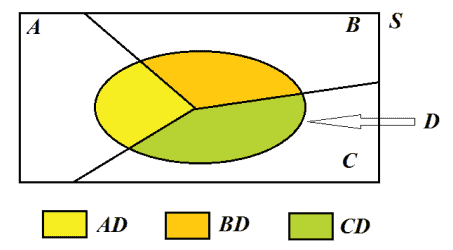
One way to perform hypothesis testing in the Bayesian framework is via the theory of Bayes factors. Suppose that on the basis of an observed event $D$ (standing for data) we wish to test a null hypothesis
$$
H_{0}: E_{0}
$$
versus an alternative hypothesis
$$
H_{1}: E_{1} \text {, }
$$
where $E_{0}$ and $E_{1}$ are two events (which are not necessarily mutually exclusive or even exhaustive of the event space).
Then we calculate:
$\pi_{0}=P\left(E_{0}\right)=$ the prior probability of the null hypothesis
$\pi_{1}=P\left(E_{1}\right)=$ the prior probability of the alternative hypothesis
$P R O=\pi_{0} / \pi_{1}=$ the prior odds in favour of the null hypothesis
$p_{0}=P\left(E_{0} \mid D\right)=$ the posterior probability of the null hypothesis
$p_{1}=P\left(E_{1} \mid D\right)=$ the posterior probability of the alternative hypothesis
$P O O=p_{0} / p_{1}=$ the posterior odds in favour of the null hypothesis.
The Bayes factor is then defined as $B F=P O O / P R O$. This may be interpreted as the factor by which the data have multiplied the odds in favour of the null hypothesis relative to the alternative hypothesis. If $B F>1$ then the data has increased the relative likelihood of the null, and if $B F<1$ then the data has decreased that relative likelihood. The magnitude of $B F$ tells us how much effect the data has had on the relative likelihood.
统计代写|贝叶斯分析代写Bayesian Analysis代考|Bayesian models
Bayes’ formula extends naturally to statistical models. A Bayesian model is a parametric model in the classical (or frequentist) sense, but with the addition of a prior probability distribution for the model parameter, which is treated as a random variable rather than an unknown constant. The basic components of a Bayesian model may be listed as:
- the data, denoted by $y$
- the parameter, denoted by $\theta$
- the model distribution, given by a specification of $f(y \mid \theta)$ or $F(y \mid \theta)$ or the distribution of $(y \mid \theta)$
- the prior distribution, given by a specification of $f(\theta)$ or $F(\theta)$ or the distribution of $\theta .$
Here, $F$ is a generic symbol which denotes cumulative distribution function (cdf), and $f$ is a generic symbol which denotes probability density function (pdf) (when applied to a continuous random variable) or probability mass function (pmf) (when applied to a discrete random variable). For simplicity, we will avoid the term pmf and use the term pdf or density for all types of random variable, including the mixed type.
Note 1: A mixed distribution is defined by a cdf which exhibits at least one discontinuity (or jump) and is strictly increasing over at least one interval of values.
Note 2: The prior may be specified by writing a statement of the form ‘ $\theta \sim \ldots$, where the symbol ‘ $\sim$ ‘ means ‘is distributed as’, and where ‘…’denotes the relevant distribution. Likewise, the model for the data may be specified by writing a statement of the form ‘ $(y \mid \theta) \sim \ldots$ ‘.
Note 3: At this stage we will not usually distinguish between $y$ as a random variable and $y$ as a value of that random variable; but sometimes we may use $Y$ for the former. Each of $y$ and $\theta$ may be a scalar, vector, matrix or array. Also, each component of $y$ and $\theta$ may have a discrete distribution, a continuous distribution, or a mixed distribution.
In the first few examples below, we will focus on the simplest case where both $y$ and $\theta$ are scalar and discrete.
贝叶斯分析代考
统计代写|贝叶斯分析代写Bayesian Analysis代考|Bayes’ rule
贝叶斯推理的起点是贝叶斯规则。最简单的形式是
磷(一个∣乙)=磷(一个)磷(乙∣一个)磷(一个)磷(乙∣一个)+磷(一个¯)磷(乙∣一个¯),
在哪里一个和乙是这样的事件磷(乙)>0. 考虑到这一点,这很容易证明:
磷(一个∣乙)=磷(一个乙)磷(乙)根据条件概率的定义磷(一个乙)=磷(一个)磷(乙∣一个)根据乘法概率定律磷(乙)=磷(一个乙)+磷(一个¯乙)=磷(一个)磷(乙∣一个)+磷(一个¯)磷(乙∣一个¯)
根据全概率定律。
我们看到后验概率磷(一个∣乙)等于先验概率磷(一个)乘以一个因子,该因子由下式给出磷(乙∣一个)/磷(乙)
关于术语,我们称磷(一个)先验概率一个(意思是概率一个前乙已知已经发生),我们称磷(一个∣乙)的后验概率一个给定乙(意思是概率一个后乙已知发生)。我们也可以说磷(一个)代表我们的先验信念一个, 和磷(一个∣乙)代表我们关于后验的信念一个.
统计代写|贝叶斯分析代写Bayesian Analysis代考|Bayes factors
在贝叶斯框架中执行假设检验的一种方法是通过贝叶斯因子理论。假设基于观察到的事件D(代表数据)我们希望检验零假设
H0:和0
与替代假设
H1:和1,
在哪里和0和和1是两个事件(它们不一定是相互排斥的,甚至不一定是事件空间的穷举)。
然后我们计算:
圆周率0=磷(和0)=原假设的先验概率
圆周率1=磷(和1)=备择假设的先验概率
磷R○=圆周率0/圆周率1=支持原假设的先验几率
p0=磷(和0∣D)=原假设的后验概率
p1=磷(和1∣D)=备择假设的后验概率
磷○○=p0/p1=支持原假设的后验概率。
贝叶斯因子然后定义为乙F=磷○○/磷R○. 这可以解释为数据乘以有利于零假设相对于备择假设的几率的因素。如果乙F>1那么数据增加了空值的相对可能性,如果乙F<1那么数据降低了这种相对可能性。的幅度乙F告诉我们数据对相对可能性的影响有多大。
统计代写|贝叶斯分析代写Bayesian Analysis代考|Bayesian models
贝叶斯公式自然地扩展到统计模型。贝叶斯模型是经典(或常客)意义上的参数模型,但增加了模型参数的先验概率分布,将其视为随机变量而不是未知常数。贝叶斯模型的基本组成部分可以列出如下:
- 数据,表示为是
- 参数,表示为θ
- 模型分布,由规范给出F(是∣θ)或者F(是∣θ)或分布(是∣θ)
- 先验分布,由规范给出F(θ)或者F(θ)或分布θ.
这里,F是表示累积分布函数 (cdf) 的通用符号,并且F是一个通用符号,表示概率密度函数 (pdf)(当应用于连续随机变量时)或概率质量函数 (pmf)(当应用于离散随机变量时)。为简单起见,我们将避免使用术语 pmf 并使用术语 pdf 或密度来表示所有类型的随机变量,包括混合类型。
注 1:混合分布由 cdf 定义,该 cdf 表现出至少一个不连续性(或跳跃)并且在至少一个值区间内严格增加。
注 2:先验可以通过编写形式为 ‘θ∼…, 其中符号 ‘∼’ 表示“分布为”,其中“……”表示相关分布。同样,数据的模型可以通过编写形式为 ‘(是∣θ)∼… ‘.
注3:在这个阶段我们通常不会区分是作为随机变量和是作为该随机变量的值;但有时我们可能会使用是对于前者。每一个是和θ可以是标量、向量、矩阵或数组。此外,每个组件是和θ可能具有离散分布、连续分布或混合分布。
在下面的前几个示例中,我们将关注最简单的情况,其中是和θ是标量和离散的。

统计代写请认准statistics-lab™. statistics-lab™为您的留学生涯保驾护航。
金融工程代写
金融工程是使用数学技术来解决金融问题。金融工程使用计算机科学、统计学、经济学和应用数学领域的工具和知识来解决当前的金融问题,以及设计新的和创新的金融产品。
非参数统计代写
非参数统计指的是一种统计方法,其中不假设数据来自于由少数参数决定的规定模型;这种模型的例子包括正态分布模型和线性回归模型。
广义线性模型代考
广义线性模型(GLM)归属统计学领域,是一种应用灵活的线性回归模型。该模型允许因变量的偏差分布有除了正态分布之外的其它分布。
术语 广义线性模型(GLM)通常是指给定连续和/或分类预测因素的连续响应变量的常规线性回归模型。它包括多元线性回归,以及方差分析和方差分析(仅含固定效应)。
有限元方法代写
有限元方法(FEM)是一种流行的方法,用于数值解决工程和数学建模中出现的微分方程。典型的问题领域包括结构分析、传热、流体流动、质量运输和电磁势等传统领域。
有限元是一种通用的数值方法,用于解决两个或三个空间变量的偏微分方程(即一些边界值问题)。为了解决一个问题,有限元将一个大系统细分为更小、更简单的部分,称为有限元。这是通过在空间维度上的特定空间离散化来实现的,它是通过构建对象的网格来实现的:用于求解的数值域,它有有限数量的点。边界值问题的有限元方法表述最终导致一个代数方程组。该方法在域上对未知函数进行逼近。[1] 然后将模拟这些有限元的简单方程组合成一个更大的方程系统,以模拟整个问题。然后,有限元通过变化微积分使相关的误差函数最小化来逼近一个解决方案。
tatistics-lab作为专业的留学生服务机构,多年来已为美国、英国、加拿大、澳洲等留学热门地的学生提供专业的学术服务,包括但不限于Essay代写,Assignment代写,Dissertation代写,Report代写,小组作业代写,Proposal代写,Paper代写,Presentation代写,计算机作业代写,论文修改和润色,网课代做,exam代考等等。写作范围涵盖高中,本科,研究生等海外留学全阶段,辐射金融,经济学,会计学,审计学,管理学等全球99%专业科目。写作团队既有专业英语母语作者,也有海外名校硕博留学生,每位写作老师都拥有过硬的语言能力,专业的学科背景和学术写作经验。我们承诺100%原创,100%专业,100%准时,100%满意。
随机分析代写
随机微积分是数学的一个分支,对随机过程进行操作。它允许为随机过程的积分定义一个关于随机过程的一致的积分理论。这个领域是由日本数学家伊藤清在第二次世界大战期间创建并开始的。
时间序列分析代写
随机过程,是依赖于参数的一组随机变量的全体,参数通常是时间。 随机变量是随机现象的数量表现,其时间序列是一组按照时间发生先后顺序进行排列的数据点序列。通常一组时间序列的时间间隔为一恒定值(如1秒,5分钟,12小时,7天,1年),因此时间序列可以作为离散时间数据进行分析处理。研究时间序列数据的意义在于现实中,往往需要研究某个事物其随时间发展变化的规律。这就需要通过研究该事物过去发展的历史记录,以得到其自身发展的规律。
回归分析代写
多元回归分析渐进(Multiple Regression Analysis Asymptotics)属于计量经济学领域,主要是一种数学上的统计分析方法,可以分析复杂情况下各影响因素的数学关系,在自然科学、社会和经济学等多个领域内应用广泛。
MATLAB代写
MATLAB 是一种用于技术计算的高性能语言。它将计算、可视化和编程集成在一个易于使用的环境中,其中问题和解决方案以熟悉的数学符号表示。典型用途包括:数学和计算算法开发建模、仿真和原型制作数据分析、探索和可视化科学和工程图形应用程序开发,包括图形用户界面构建MATLAB 是一个交互式系统,其基本数据元素是一个不需要维度的数组。这使您可以解决许多技术计算问题,尤其是那些具有矩阵和向量公式的问题,而只需用 C 或 Fortran 等标量非交互式语言编写程序所需的时间的一小部分。MATLAB 名称代表矩阵实验室。MATLAB 最初的编写目的是提供对由 LINPACK 和 EISPACK 项目开发的矩阵软件的轻松访问,这两个项目共同代表了矩阵计算软件的最新技术。MATLAB 经过多年的发展,得到了许多用户的投入。在大学环境中,它是数学、工程和科学入门和高级课程的标准教学工具。在工业领域,MATLAB 是高效研究、开发和分析的首选工具。MATLAB 具有一系列称为工具箱的特定于应用程序的解决方案。对于大多数 MATLAB 用户来说非常重要,工具箱允许您学习和应用专业技术。工具箱是 MATLAB 函数(M 文件)的综合集合,可扩展 MATLAB 环境以解决特定类别的问题。可用工具箱的领域包括信号处理、控制系统、神经网络、模糊逻辑、小波、仿真等。