如果你也在 怎样代写贝叶斯分析Bayesian Analysis这个学科遇到相关的难题,请随时右上角联系我们的24/7代写客服。
贝叶斯分析,一种统计推断方法(以英国数学家托马斯-贝叶斯命名),允许人们将关于人口参数的先验信息与样本所含信息的证据相结合,以指导统计推断过程。
statistics-lab™ 为您的留学生涯保驾护航 在代写贝叶斯分析Bayesian Analysis方面已经树立了自己的口碑, 保证靠谱, 高质且原创的统计Statistics代写服务。我们的专家在代写贝叶斯分析Bayesian Analysis代写方面经验极为丰富,各种代写贝叶斯分析Bayesian Analysis相关的作业也就用不着说。
我们提供的贝叶斯分析Bayesian Analysis及其相关学科的代写,服务范围广, 其中包括但不限于:
- Statistical Inference 统计推断
- Statistical Computing 统计计算
- Advanced Probability Theory 高等概率论
- Advanced Mathematical Statistics 高等数理统计学
- (Generalized) Linear Models 广义线性模型
- Statistical Machine Learning 统计机器学习
- Longitudinal Data Analysis 纵向数据分析
- Foundations of Data Science 数据科学基础
统计代写|贝叶斯分析代写Bayesian Analysis代考|The posterior expected loss
We have defined the risk function as the expectation of the loss function given the parameter, namely
$$
R(\theta)=E(L(\hat{\theta}, \theta) \mid \theta)=\int L(\hat{\theta}(y), \theta) f(y \mid \theta) d y .
$$
Conversely, we now define the posterior expected loss (PEL) as the expectation of the loss function given the data, and we denote this function by
$$
P E L(y)=E{L(\hat{\theta}, \theta) \mid y}=\int L(\hat{\theta}(y), \theta) f(\theta \mid y) d \theta .
$$
Then, just as the risk function can be used to compute the Bayes risk according to
$$
r=E L(\hat{\theta}, \theta)=E E{L(\hat{\theta}, \theta) \mid \theta}=E R(\theta)=\int R(\theta) f(\theta) d \theta,
$$
so also can the PEL be used, but with the formula
$$
r=E L(\hat{\theta}, \theta)=E E{L(\hat{\theta}, \theta) \mid y}=E{P E L(y)}=\int \operatorname{PEL}(y) f(y) d y .
$$
Note: Both of these formulae for the Bayes risk use the law of iterated expectation, but with different conditionings.
统计代写|贝叶斯分析代写Bayesian Analysis代考|The Bayes estimate
The Bayes estimate (or estimator) is defined to be the choice of the function $\hat{\theta}=\hat{\theta}(y)$ for which the Bayes risk $r=E L(\hat{\theta}, \theta)$ is minimised. This estimator has the smallest overall expected loss over all estimators under the specified loss function $L(\hat{\theta}, \theta)$.
In many cases, the procedure for finding a Bayes estimate can be considerably simplified by considering which estimate minimises the posterior expected loss function, $P E L(y)=E{L(\hat{\theta}, \theta) \mid y}$.
If we can find an estimate $\hat{\theta}=\hat{\theta}(y)$ which minimises $\operatorname{PEL}(y)$ for all possible values of the data $y$, then that estimate must also minimise the Bayes risk.
This is because the Bayes risk may be written as a weighted average of the PEL, namely
$$
r=E L(\hat{\theta}, \theta)=E E{L(\hat{\theta}, \theta) \mid y}=E{P E L(y)}=\int \operatorname{PEL}(y) f(y) d y .
$$
Exercise 2.10 Bayes estimate under the QELF
Find the Bayes estimate under the quadratic error loss function.
Solution to Exercise 2.10
$$
\text { Observe that } \quad \begin{aligned}
P E L(y) &=E\left{(\hat{\theta}-\theta)^{2} \mid y\right}=E\left{\hat{\theta}^{2}-2 \hat{\theta} \theta+\theta^{2} \mid y\right} \
&=\hat{\theta}^{2}-2 \hat{\theta} E(\theta \mid y)+E\left(\theta^{2} \mid y\right) \
&=[\hat{\theta}-E(\theta \mid y)]^{2}-{E(\theta \mid y)}^{2}+E\left(\theta^{2} \mid y\right)
\end{aligned}
$$
Note: We have completed the square in $\hat{\theta}$.
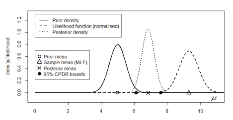
We see that the PEL is a quadratic function of $\hat{\theta}$ which is clearly minimised at the posterior mean, $\hat{\theta}=E(\theta \mid y)$. So the Bayes estimate under the QELF is that posterior mean.
统计代写|贝叶斯分析代写Bayesian Analysis代考|Inference given functions of the data
Sometimes we observe a function of the data rather than the data itself. In such cases the function typically degrades the information available in some way. An example is censoring, where we observe a value only if that value is less than some cut-off point (right censoring) or greater than some cut-off value (left censoring). It is also possible to have censoring on the left and right simultaneously. Another example is rounding, where we only observe values to the nearest multiple of $0.1,1$ or 5 , etc.
Exercise 3.I Right censoring of exponential observations
Each light bulb of a certain type has a life which is conditionally exponential with mean $m=1 / c$, where $c$ has a prior distribution which is standard exponential. We observe $n=5$ light bulbs of this type for 6 units of time, and the lifetimes are:
$$
2.6,3.2, *, 1.2 \text {, * }
$$
where $*$ indicates a right-censored value which is greater than 6 . (Only values less than or equal to 6 could be observed.)
Find the posterior distribution and mean of the average light bulb lifetime, $m$.
The data here is
$$
D=\left{y_{1}=2.6, y_{2}=3.2, y_{3}>6, y_{4}=1.2, y_{5}>6\right} \text {, }
$$
and the probability of censoring is
$$
P\left(y_{i}>6 \mid c\right)=\int_{6}^{\infty} c e^{-c y_{i}} d y_{i}=e^{-6 c} .
$$
Therefore the posterior density of $c$ is
$$
\begin{aligned}
f(c \mid D) & \propto f(c) f(D \mid c) \
& \propto f(c) f\left(y_{1} \mid c\right) f\left(y_{2} \mid c\right) P\left(y_{3}>6 \mid c\right) f\left(y_{4} \mid c\right) P\left(y_{5}>6 \mid c\right)
\end{aligned}
$$ $$
\begin{aligned}
&\propto e^{-c}\left(c e^{-c c_{1}}\right)\left(c e^{-c y_{2}}\right)\left(e^{-6 c}\right)\left(c e^{-c y_{4}}\right)\left(e^{-6 c}\right) \
&=c^{3} \exp \left{-c\left(1+y_{1}+y_{2}+6+y_{4}+6\right)\right} \
&=c^{4-1} \exp {-c(1+2.6+3.2+6+1.2+6)} \
&=c^{4-1} \exp (-20 c)
\end{aligned}
$$
Hence:
$$
\begin{aligned}
&(c \mid D) \sim G(4,20) \
&(m \mid D) \sim I G(4,20) \
&f(m \mid D)=20^{4} m^{-(4+1)} e^{-20 / m} / \Gamma(4), m>0 \
&E(m \mid D)=20 /(4-1)=6.667
\end{aligned}
$$
It will be observed that this estimate of $m$ is appropriately higher than the estimate obtained by simply averaging the observed values, namely
$$
(1 / 3)(2.6+3.2+1.2)=2.333 \text {. }
$$
The estimate $6.667$ is also higher than the estimate obtained by simply replacing the censored values with 6 , namely
$$
(1 / 3)(2.6+3.2+6+1.2+6)=3.8 \text {. }
$$
贝叶斯分析代考
统计代写|贝叶斯分析代写Bayesian Analysis代考|The posterior expected loss
我们将风险函数定义为给定参数的损失函数的期望值,即
R(θ)=和(大号(θ^,θ)∣θ)=∫大号(θ^(是),θ)F(是∣θ)d是.
相反,我们现在将后验期望损失(PEL)定义为给定数据的损失函数的期望,我们将这个函数表示为
磷和大号(是)=和大号(θ^,θ)∣是=∫大号(θ^(是),θ)F(θ∣是)dθ.
然后,就像风险函数可以用来计算贝叶斯风险一样
r=和大号(θ^,θ)=和和大号(θ^,θ)∣θ=和R(θ)=∫R(θ)F(θ)dθ,
所以也可以使用 PEL,但使用公式
r=和大号(θ^,θ)=和和大号(θ^,θ)∣是=和磷和大号(是)=∫佩尔(是)F(是)d是.
注意:这两个贝叶斯风险公式都使用了迭代期望定律,但条件不同。
统计代写|贝叶斯分析代写Bayesian Analysis代考|The Bayes estimate
贝叶斯估计(或估计器)被定义为函数的选择θ^=θ^(是)贝叶斯风险r=和大号(θ^,θ)被最小化。在指定损失函数下,该估计器在所有估计器中具有最小的总体预期损失大号(θ^,θ).
在许多情况下,通过考虑哪个估计最小化后验期望损失函数,可以大大简化寻找贝叶斯估计的过程,磷和大号(是)=和大号(θ^,θ)∣是.
如果我们能找到一个估计θ^=θ^(是)最小化佩尔(是)对于数据的所有可能值是,那么该估计也必须最小化贝叶斯风险。
这是因为贝叶斯风险可以写成 PEL 的加权平均值,即
r=和大号(θ^,θ)=和和大号(θ^,θ)∣是=和磷和大号(是)=∫佩尔(是)F(是)d是.
练习 2.10 QELF 下
的贝叶斯估计 求二次误差损失函数下的贝叶斯估计。
习题 2.10 的解法
\text { 观察到 } \quad \begin{aligned} P E L(y) &=E\left{(\hat{\theta}-\theta)^{2} \mid y\right}=E\left{\帽子{\theta}^{2}-2 \hat{\theta} \theta+\theta^{2} \mid y\right} \ &=\hat{\theta}^{2}-2 \hat{\ theta} E(\theta \mid y)+E\left(\theta^{2} \mid y\right) \ &=[\hat{\theta}-E(\theta \mid y)]^{2 }-{E(\theta \mid y)}^{2}+E\left(\theta^{2} \mid y\right) \end{对齐}\text { 观察到 } \quad \begin{aligned} P E L(y) &=E\left{(\hat{\theta}-\theta)^{2} \mid y\right}=E\left{\帽子{\theta}^{2}-2 \hat{\theta} \theta+\theta^{2} \mid y\right} \ &=\hat{\theta}^{2}-2 \hat{\ theta} E(\theta \mid y)+E\left(\theta^{2} \mid y\right) \ &=[\hat{\theta}-E(\theta \mid y)]^{2 }-{E(\theta \mid y)}^{2}+E\left(\theta^{2} \mid y\right) \end{对齐}
注意:我们已经完成了广场θ^.
我们看到 PEL 是一个二次函数θ^在后验均值处明显最小化,θ^=和(θ∣是). 所以 QELF 下的贝叶斯估计就是后验均值。
统计代写|贝叶斯分析代写Bayesian Analysis代考|Inference given functions of the data
有时我们观察的是数据的函数而不是数据本身。在这种情况下,该功能通常会以某种方式降低可用信息的质量。一个例子是审查,只有当该值小于某个截止点(右删失)或大于某个截止值(左删失)时,我们才观察该值。也可以同时对左右进行审查。另一个例子是四舍五入,我们只观察到最接近的倍数的值0.1,1
or
5等米=1/C, 在哪里C具有标准指数的先验分布。我们观察n=5此类灯泡可使用 6 个单位时间,其寿命为:
2.6,3.2,∗,1.2, *
在哪里∗表示大于 6 的右删失值。(只能观察到小于或等于 6 的值。)
求灯泡平均寿命的后验分布和均值,米.
这里的数据是
D=\left{y_{1}=2.6, y_{2}=3.2, y_{3}>6, y_{4}=1.2, y_{5}>6\right} \text {, }D=\left{y_{1}=2.6, y_{2}=3.2, y_{3}>6, y_{4}=1.2, y_{5}>6\right} \text {, }
审查的概率是
磷(是一世>6∣C)=∫6∞C和−C是一世d是一世=和−6C.
因此后验密度C是
F(C∣D)∝F(C)F(D∣C) ∝F(C)F(是1∣C)F(是2∣C)磷(是3>6∣C)F(是4∣C)磷(是5>6∣C)
\begin{aligned} &\propto e^{-c}\left(c e^{-c c_{1}}\right)\left(c e^{-c y_{2}}\right)\left(e ^{-6 c}\right)\left(c e^{-c y_{4}}\right)\left(e^{-6 c}\right) \ &=c^{3} \exp \left {-c\left(1+y_{1}+y_{2}+6+y_{4}+6\right)\right} \ &=c^{4-1} \exp {-c(1+ 2.6+3.2+6+1.2+6)} \ &=c^{4-1} \exp (-20 c) \end{对齐}\begin{aligned} &\propto e^{-c}\left(c e^{-c c_{1}}\right)\left(c e^{-c y_{2}}\right)\left(e ^{-6 c}\right)\left(c e^{-c y_{4}}\right)\left(e^{-6 c}\right) \ &=c^{3} \exp \left {-c\left(1+y_{1}+y_{2}+6+y_{4}+6\right)\right} \ &=c^{4-1} \exp {-c(1+ 2.6+3.2+6+1.2+6)} \ &=c^{4-1} \exp (-20 c) \end{对齐}
因此:
(C∣D)∼G(4,20) (米∣D)∼我G(4,20) F(米∣D)=204米−(4+1)和−20/米/Γ(4),米>0 和(米∣D)=20/(4−1)=6.667
可以看出,这个估计米适当地高于通过简单地平均观察值获得的估计值,即
(1/3)(2.6+3.2+1.2)=2.333.
估计6.667也高于通过简单地将删失值替换为 6 获得的估计值,即
(1/3)(2.6+3.2+6+1.2+6)=3.8.

统计代写请认准statistics-lab™. statistics-lab™为您的留学生涯保驾护航。
金融工程代写
金融工程是使用数学技术来解决金融问题。金融工程使用计算机科学、统计学、经济学和应用数学领域的工具和知识来解决当前的金融问题,以及设计新的和创新的金融产品。
非参数统计代写
非参数统计指的是一种统计方法,其中不假设数据来自于由少数参数决定的规定模型;这种模型的例子包括正态分布模型和线性回归模型。
广义线性模型代考
广义线性模型(GLM)归属统计学领域,是一种应用灵活的线性回归模型。该模型允许因变量的偏差分布有除了正态分布之外的其它分布。
术语 广义线性模型(GLM)通常是指给定连续和/或分类预测因素的连续响应变量的常规线性回归模型。它包括多元线性回归,以及方差分析和方差分析(仅含固定效应)。
有限元方法代写
有限元方法(FEM)是一种流行的方法,用于数值解决工程和数学建模中出现的微分方程。典型的问题领域包括结构分析、传热、流体流动、质量运输和电磁势等传统领域。
有限元是一种通用的数值方法,用于解决两个或三个空间变量的偏微分方程(即一些边界值问题)。为了解决一个问题,有限元将一个大系统细分为更小、更简单的部分,称为有限元。这是通过在空间维度上的特定空间离散化来实现的,它是通过构建对象的网格来实现的:用于求解的数值域,它有有限数量的点。边界值问题的有限元方法表述最终导致一个代数方程组。该方法在域上对未知函数进行逼近。[1] 然后将模拟这些有限元的简单方程组合成一个更大的方程系统,以模拟整个问题。然后,有限元通过变化微积分使相关的误差函数最小化来逼近一个解决方案。
tatistics-lab作为专业的留学生服务机构,多年来已为美国、英国、加拿大、澳洲等留学热门地的学生提供专业的学术服务,包括但不限于Essay代写,Assignment代写,Dissertation代写,Report代写,小组作业代写,Proposal代写,Paper代写,Presentation代写,计算机作业代写,论文修改和润色,网课代做,exam代考等等。写作范围涵盖高中,本科,研究生等海外留学全阶段,辐射金融,经济学,会计学,审计学,管理学等全球99%专业科目。写作团队既有专业英语母语作者,也有海外名校硕博留学生,每位写作老师都拥有过硬的语言能力,专业的学科背景和学术写作经验。我们承诺100%原创,100%专业,100%准时,100%满意。
随机分析代写
随机微积分是数学的一个分支,对随机过程进行操作。它允许为随机过程的积分定义一个关于随机过程的一致的积分理论。这个领域是由日本数学家伊藤清在第二次世界大战期间创建并开始的。
时间序列分析代写
随机过程,是依赖于参数的一组随机变量的全体,参数通常是时间。 随机变量是随机现象的数量表现,其时间序列是一组按照时间发生先后顺序进行排列的数据点序列。通常一组时间序列的时间间隔为一恒定值(如1秒,5分钟,12小时,7天,1年),因此时间序列可以作为离散时间数据进行分析处理。研究时间序列数据的意义在于现实中,往往需要研究某个事物其随时间发展变化的规律。这就需要通过研究该事物过去发展的历史记录,以得到其自身发展的规律。
回归分析代写
多元回归分析渐进(Multiple Regression Analysis Asymptotics)属于计量经济学领域,主要是一种数学上的统计分析方法,可以分析复杂情况下各影响因素的数学关系,在自然科学、社会和经济学等多个领域内应用广泛。
MATLAB代写
MATLAB 是一种用于技术计算的高性能语言。它将计算、可视化和编程集成在一个易于使用的环境中,其中问题和解决方案以熟悉的数学符号表示。典型用途包括:数学和计算算法开发建模、仿真和原型制作数据分析、探索和可视化科学和工程图形应用程序开发,包括图形用户界面构建MATLAB 是一个交互式系统,其基本数据元素是一个不需要维度的数组。这使您可以解决许多技术计算问题,尤其是那些具有矩阵和向量公式的问题,而只需用 C 或 Fortran 等标量非交互式语言编写程序所需的时间的一小部分。MATLAB 名称代表矩阵实验室。MATLAB 最初的编写目的是提供对由 LINPACK 和 EISPACK 项目开发的矩阵软件的轻松访问,这两个项目共同代表了矩阵计算软件的最新技术。MATLAB 经过多年的发展,得到了许多用户的投入。在大学环境中,它是数学、工程和科学入门和高级课程的标准教学工具。在工业领域,MATLAB 是高效研究、开发和分析的首选工具。MATLAB 具有一系列称为工具箱的特定于应用程序的解决方案。对于大多数 MATLAB 用户来说非常重要,工具箱允许您学习和应用专业技术。工具箱是 MATLAB 函数(M 文件)的综合集合,可扩展 MATLAB 环境以解决特定类别的问题。可用工具箱的领域包括信号处理、控制系统、神经网络、模糊逻辑、小波、仿真等。