如果你也在 怎样代写贝叶斯统计这个学科遇到相关的难题,请随时右上角联系我们的24/7代写客服。
贝叶斯统计学是一个使用概率的数学语言来描述认识论的不确定性的系统。在 “贝叶斯范式 “中,对自然状态的相信程度是明确的;这些程度是非负的,而对所有自然状态的总相信是固定的。
statistics-lab™ 为您的留学生涯保驾护航 在代写贝叶斯统计方面已经树立了自己的口碑, 保证靠谱, 高质且原创的统计Statistics代写服务。我们的专家在代写贝叶斯统计代写方面经验极为丰富,各种代写贝叶斯统计相关的作业也就用不着说。
我们提供的贝叶斯统计及其相关学科的代写,服务范围广, 其中包括但不限于:
- Statistical Inference 统计推断
- Statistical Computing 统计计算
- Advanced Probability Theory 高等概率论
- Advanced Mathematical Statistics 高等数理统计学
- (Generalized) Linear Models 广义线性模型
- Statistical Machine Learning 统计机器学习
- Longitudinal Data Analysis 纵向数据分析
- Foundations of Data Science 数据科学基础
统计代写|贝叶斯统计代写beyesian statistics代考|Spatio-temporal data types
Data are called spatio-temporal as long as each one of them carries a location and a time stamp. This leaves open the possibility of a huge number of spatio-temporal data types even if we exclude the two extreme degenerate possibilities where data are observed either at a single point of time or at a single location in space. Analysts often opt for one of the two degenerate possibilities when they are not interested in the variation due to either space or time. This may simply be achieved by suitably aggregating the variation in the ignored category. For example, one may report the annual average air pollution levels at different monitoring sites in a network when daily data are available. Aggregating over time or space reduces variability in the data to be analyzed and will also limit the extent of inferences that can be made. For example, it is not possible to detect or apportion monthly trends just by analyzing annual aggregates. This text book will assume that there is spatiotemporal variation in the data, although it will discuss important concepts, as required, for studying spatial or temporal only data.
One of the very first tasks in analyzing spatio-temporal data is to choose the spatial and temporal resolutions at which to model the data. The main issues to consider are the inferential objectives of the study. Here one needs to decide the highest possible spatial and temporal resolutions at which inferences must be made. Such considerations will largely determine whether we are required to work with daily, monthly or annual data, for example. There are other issues at stake here as well. For example, relationships between variables may be understood better at a finer resolution than a coarser resolution, e.g. hourly air pollution level may have a stronger relationship with hourly wind speed than what the annual average air pollution level will have with the annual average wind speed. Thus, aggregation may lead to correlation degradation. However, too fine a resolution, either temporal and/or spatial, may pose a huge challenge in data processing, modeling and analysis without adding much extra information. Thus, a balance needs to be stuck when deciding on the spatio-temporal resolution of the data to be analyzed and modeled. These decisions must be taken at the data pre-processing stage before formal modeling and analysis can begin.
Suppose that the temporal resolution of the data has been decided, and we use the symbol $t$ to denote each time point and we suppose that there are $T$ regularly spaced time points in total. This is a restrictive assumption as often there are cases of irregularly spaced temporal data. For example, a patient may be followed up at different time intervals; there may be missed appointments during a schedule of regular check-ups. In an air pollution monitoring example, there may be more monitoring performed during episodes of high air pollution. For example, it may be necessary to decide whether to model air pollution at an hourly or daily time scales. In such situations, depending on the main purposes of the study, there are two main strategies for modeling. The first one is to model at the highest possible regular temporal resolution, in which case there would be many missing observations for all the unobserved time points. Modeling will help estimate those missing observations and their uncertainties. For example, modeling air pollution at the hourly resolution will lead to missing observations for all the unmonitored hours. The second strategy avoiding the many missing observations of the first strategy is to model at an aggregated temporal resolution where all the available observations within a regular time window are suitably averaged to arrive at the observation that will correspond to that aggregated time. For example, all the observed hourly air pollution recordings are averaged to arrive at the daily average air pollution value. Although this strategy is successful in avoiding many missing observations, there may still be challenges in modeling since the aggregated response values may show un-equal variances since those have been obtained from different numbers of observations during the aggregated time windows. In summary, careful considerations are required to select the temporal resolution for modeling.
统计代写|贝叶斯统计代写beyesian statistics代考|New York air pollution data set
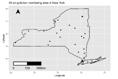
We use a real-life data set, previously analyzed by Sahu and Bakar (2012a), on daily maximum 8-hour average ground-level ozone concentration for the months of July and August in 2006 , observed at 28 monitoring sites in the state of New York. We consider three important covariates: maximum temperature (xmaxtemp in degree Celsius), wind speed (xwdsp in nautical miles), and percentage average relative humidity (xrh) for building a spatiotemporal model for ozone concentration. Further details regarding the covariate values and their spatial interpolations for prediction purposes are provided in Bakar (2012). This data set is available as the data frame nysptime in the bmstdr package. The data set has 12 columns and 1736 rows. The $R$ help command ?nysptime provides detailed description for the columns.
In this book we will also use a temporally aggregated spatial version of this data set. Available as the data set nyspatial in the bmstdr package, it has data for 28 sites in 28 rows and 9 columns. The $R$ help command ?nyspatial provides detailed descriptions for the columns. Values of the response and the covariates in this data set are simple averages (after removing the missing observations) of the corresponding columns in nysptime. Figure $1.1$ represents a map of the state of New York together with the 28 monitoring locations.The two data sets nyspatial and nysptime will be used as running examples for all the point referenced data models in Chapters 6 and 7. The spatiotemporal data set nysptime is also used to illustrate forecasting in Chapter 9 . Chapter 3 provides some preliminary exploratory analysis of these two data sets.
统计代写|贝叶斯统计代写beyesian statistics代考|Air pollution data from England and Wales
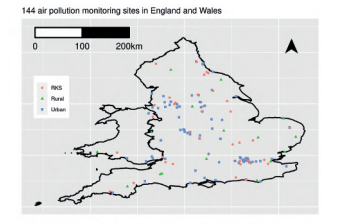
This example illustrates the modeling of daily mean concentrations of nitrogen dioxide $\left(\mathrm{NO}{2}\right)$, ozone $\left(\mathrm{O}{3}\right)$ and particles less than $10 \mu m\left(\mathrm{PM}{10}\right)$ and $2.5 \mu m$ $\left(\mathrm{PM}{2.5}\right)$ which were obtained from $n=144$ locations from the Automatic Urban and Rural Network (AURN, http://uk-air.defra.gov.uk/networks) in England and Wales. The 144 locations are categorized into three site types: rural (16), urban (81) and RKS (Road amd Kerb Side) (47). The locations of these 144 sites are shown in Figure 1.2.
Mukhopadhyay and Sahu (2018) analyze this data set comprehensively and obtain aggregated annual predictions at each of the local and unitary authorities in England and Wales. It takes an enormous amount of computing effort and data processing to reproduce the work done by Mukhopadhyay and Sahu (2018) and as a result, we do not attempt this here. Instead, we illustrate spatio-temporal modeling for $\mathrm{NO}_{2}$ for 365 days in the year 2011 . We also obtain an annual average prediction map based on modeling of the daily data in Section 8.2.
贝叶斯统计代写
统计代写|贝叶斯统计代写beyesian statistics代考|Spatio-temporal data types
只要数据中的每一个都带有位置和时间戳,就称为时空数据。即使我们排除了在单个时间点或在空间中的单个位置观察到数据的两种极端退化的可能性,这也为大量时空数据类型留下了可能性。当分析师对空间或时间的变化不感兴趣时,他们通常会选择两种退化可能性之一。这可以通过适当地聚合忽略类别中的变化来简单地实现。例如,当每日数据可用时,可以报告网络中不同监测点的年平均空气污染水平。随时间或空间进行的聚合减少了要分析的数据的可变性,并且还将限制可以做出的推断的范围。例如,仅通过分析年度总量是不可能发现或分配每月趋势的。这本书将假设数据存在时空变化,尽管它会根据需要讨论研究空间或时间数据的重要概念。
分析时空数据的首要任务之一是选择对数据建模的空间和时间分辨率。要考虑的主要问题是研究的推理目标。在这里,需要确定必须进行推断的最高可能的空间和时间分辨率。例如,这些考虑将在很大程度上决定我们是否需要处理每日、每月或每年的数据。这里还有其他问题。例如,在较精细的分辨率下,变量之间的关系可能比在较粗的分辨率下更好地理解,例如,每小时空气污染水平与每小时风速的关系可能比年平均空气污染水平与年平均风速的关系更强。因此,聚合可能导致相关性退化。然而,太精细的分辨率,无论是时间和/或空间,都可能在不添加太多额外信息的情况下对数据处理、建模和分析造成巨大挑战。因此,在决定要分析和建模的数据的时空分辨率时,需要保持平衡。这些决定必须在正式建模和分析开始之前的数据预处理阶段做出。
假设数据的时间分辨率已经确定,我们使用符号吨来表示每个时间点,我们假设有吨总共有规律地间隔的时间点。这是一个限制性假设,因为经常存在不规则间隔的时间数据的情况。例如,可以在不同的时间间隔对患者进行随访;在定期检查期间可能会错过约会。在空气污染监测示例中,在高空气污染期间可能会执行更多监测。例如,可能需要决定是按小时还是按天时间尺度模拟空气污染。在这种情况下,根据研究的主要目的,有两种主要的建模策略。第一个是以尽可能高的常规时间分辨率建模,在这种情况下,所有未观察到的时间点都会有很多缺失的观察结果。建模将有助于估计那些缺失的观测值及其不确定性。例如,以小时分辨率模拟空气污染将导致所有未监测时间的观测结果丢失。避免第一种策略的许多缺失观测值的第二种策略是以聚合时间分辨率进行建模,其中在常规时间窗口内的所有可用观测值都被适当地平均以得出与该聚合时间相对应的观测值。例如,将所有观察到的每小时空气污染记录进行平均,以得出每日平均空气污染值。尽管这种策略成功地避免了许多缺失的观察结果,建模可能仍然存在挑战,因为聚合响应值可能显示出不相等的方差,因为这些值是从聚合时间窗口内不同数量的观察中获得的。总之,需要仔细考虑选择用于建模的时间分辨率。
统计代写|贝叶斯统计代写beyesian statistics代考|New York air pollution data set
我们使用 Sahu 和 Bakar (2012a) 之前分析的真实数据集,该数据集是 2006 年 7 月和 8 月在 28 个监测点观察到的每日最大 8 小时平均地面臭氧浓度。纽约。我们考虑三个重要的协变量:最高温度(以摄氏度为单位的 xmaxtemp)、风速(以海里为单位的 xwdsp)和平均相对湿度百分比(xrh),以构建臭氧浓度的时空模型。Bakar (2012) 中提供了有关协变量值及其用于预测目的的空间插值的更多详细信息。此数据集可用作 bmstdr 包中的数据帧 nysptime。数据集有 12 列和 1736 行。这R帮助命令 ?nysptime 提供列的详细说明。
在本书中,我们还将使用该数据集的时间聚合空间版本。作为 bmstdr 包中的数据集 nyspatial 可用,它包含 28 行和 9 列中的 28 个站点的数据。这Rhelp command ?nyspatial 提供了列的详细描述。该数据集中的响应值和协变量是 nysptime 中相应列的简单平均值(在删除缺失的观察值之后)。数字1.1表示纽约州连同 28 个监测点的地图。这两个数据集 nyspatial 和 nysptime 将用作第 6 章和第 7 章中所有点引用数据模型的运行示例。时空数据集 nysptime 也被使用在第 9 章中说明预测。第 3 章对这两个数据集进行了一些初步的探索性分析。
统计代写|贝叶斯统计代写beyesian statistics代考|Air pollution data from England and Wales
这个例子说明了二氧化氮日平均浓度的建模(ñ这2), 臭氧(这3)并且颗粒小于10μ米(磷米10)和2.5μ米 (磷米2.5)获得自n=144来自英格兰和威尔士的自动城乡网络 (AURN, http://uk-air.defra.gov.uk/networks) 的位置。144 个地点分为三种场地类型:农村 (16)、城市 (81) 和 RKS(路边和路边)(47)。这 144 个站点的位置如图 1.2 所示。
Mukhopadhyay 和 Sahu(2018 年)全面分析了该数据集,并获得了英格兰和威尔士每个地方和单一当局的汇总年度预测。重现 Mukhopadhyay 和 Sahu (2018) 所做的工作需要大量的计算工作和数据处理,因此,我们不在这里尝试。相反,我们说明时空建模ñ这22011 年 365 天。我们还根据第 8.2 节中的每日数据建模获得了年平均预测图。

统计代写请认准statistics-lab™. statistics-lab™为您的留学生涯保驾护航。
金融工程代写
金融工程是使用数学技术来解决金融问题。金融工程使用计算机科学、统计学、经济学和应用数学领域的工具和知识来解决当前的金融问题,以及设计新的和创新的金融产品。
非参数统计代写
非参数统计指的是一种统计方法,其中不假设数据来自于由少数参数决定的规定模型;这种模型的例子包括正态分布模型和线性回归模型。
广义线性模型代考
广义线性模型(GLM)归属统计学领域,是一种应用灵活的线性回归模型。该模型允许因变量的偏差分布有除了正态分布之外的其它分布。
术语 广义线性模型(GLM)通常是指给定连续和/或分类预测因素的连续响应变量的常规线性回归模型。它包括多元线性回归,以及方差分析和方差分析(仅含固定效应)。
有限元方法代写
有限元方法(FEM)是一种流行的方法,用于数值解决工程和数学建模中出现的微分方程。典型的问题领域包括结构分析、传热、流体流动、质量运输和电磁势等传统领域。
有限元是一种通用的数值方法,用于解决两个或三个空间变量的偏微分方程(即一些边界值问题)。为了解决一个问题,有限元将一个大系统细分为更小、更简单的部分,称为有限元。这是通过在空间维度上的特定空间离散化来实现的,它是通过构建对象的网格来实现的:用于求解的数值域,它有有限数量的点。边界值问题的有限元方法表述最终导致一个代数方程组。该方法在域上对未知函数进行逼近。[1] 然后将模拟这些有限元的简单方程组合成一个更大的方程系统,以模拟整个问题。然后,有限元通过变化微积分使相关的误差函数最小化来逼近一个解决方案。
tatistics-lab作为专业的留学生服务机构,多年来已为美国、英国、加拿大、澳洲等留学热门地的学生提供专业的学术服务,包括但不限于Essay代写,Assignment代写,Dissertation代写,Report代写,小组作业代写,Proposal代写,Paper代写,Presentation代写,计算机作业代写,论文修改和润色,网课代做,exam代考等等。写作范围涵盖高中,本科,研究生等海外留学全阶段,辐射金融,经济学,会计学,审计学,管理学等全球99%专业科目。写作团队既有专业英语母语作者,也有海外名校硕博留学生,每位写作老师都拥有过硬的语言能力,专业的学科背景和学术写作经验。我们承诺100%原创,100%专业,100%准时,100%满意。
随机分析代写
随机微积分是数学的一个分支,对随机过程进行操作。它允许为随机过程的积分定义一个关于随机过程的一致的积分理论。这个领域是由日本数学家伊藤清在第二次世界大战期间创建并开始的。
时间序列分析代写
随机过程,是依赖于参数的一组随机变量的全体,参数通常是时间。 随机变量是随机现象的数量表现,其时间序列是一组按照时间发生先后顺序进行排列的数据点序列。通常一组时间序列的时间间隔为一恒定值(如1秒,5分钟,12小时,7天,1年),因此时间序列可以作为离散时间数据进行分析处理。研究时间序列数据的意义在于现实中,往往需要研究某个事物其随时间发展变化的规律。这就需要通过研究该事物过去发展的历史记录,以得到其自身发展的规律。
回归分析代写
多元回归分析渐进(Multiple Regression Analysis Asymptotics)属于计量经济学领域,主要是一种数学上的统计分析方法,可以分析复杂情况下各影响因素的数学关系,在自然科学、社会和经济学等多个领域内应用广泛。
MATLAB代写
MATLAB 是一种用于技术计算的高性能语言。它将计算、可视化和编程集成在一个易于使用的环境中,其中问题和解决方案以熟悉的数学符号表示。典型用途包括:数学和计算算法开发建模、仿真和原型制作数据分析、探索和可视化科学和工程图形应用程序开发,包括图形用户界面构建MATLAB 是一个交互式系统,其基本数据元素是一个不需要维度的数组。这使您可以解决许多技术计算问题,尤其是那些具有矩阵和向量公式的问题,而只需用 C 或 Fortran 等标量非交互式语言编写程序所需的时间的一小部分。MATLAB 名称代表矩阵实验室。MATLAB 最初的编写目的是提供对由 LINPACK 和 EISPACK 项目开发的矩阵软件的轻松访问,这两个项目共同代表了矩阵计算软件的最新技术。MATLAB 经过多年的发展,得到了许多用户的投入。在大学环境中,它是数学、工程和科学入门和高级课程的标准教学工具。在工业领域,MATLAB 是高效研究、开发和分析的首选工具。MATLAB 具有一系列称为工具箱的特定于应用程序的解决方案。对于大多数 MATLAB 用户来说非常重要,工具箱允许您学习和应用专业技术。工具箱是 MATLAB 函数(M 文件)的综合集合,可扩展 MATLAB 环境以解决特定类别的问题。可用工具箱的领域包括信号处理、控制系统、神经网络、模糊逻辑、小波、仿真等。