如果你也在 怎样代写贝叶斯网络Bayesian network这个学科遇到相关的难题,请随时右上角联系我们的24/7代写客服。
贝叶斯网络(BN)是一种表示不确定领域知识的概率图形模型,其中每个节点对应一个随机变量,每条边代表相应随机变量的条件概率。
statistics-lab™ 为您的留学生涯保驾护航 在代写贝叶斯网络Bayesian network方面已经树立了自己的口碑, 保证靠谱, 高质且原创的统计Statistics代写服务。我们的专家在代写贝叶斯网络Bayesian network代写方面经验极为丰富,各种代写贝叶斯网络Bayesian network相关的作业也就用不着说。
我们提供的贝叶斯网络Bayesian network及其相关学科的代写,服务范围广, 其中包括但不限于:
- Statistical Inference 统计推断
- Statistical Computing 统计计算
- Advanced Probability Theory 高等概率论
- Advanced Mathematical Statistics 高等数理统计学
- (Generalized) Linear Models 广义线性模型
- Statistical Machine Learning 统计机器学习
- Longitudinal Data Analysis 纵向数据分析
- Foundations of Data Science 数据科学基础
统计代写|贝叶斯网络代写Bayesian network代考|What is Spatial Time Series Data
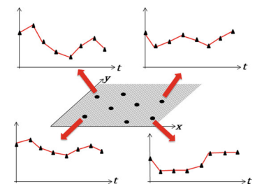
Spatial time series data is a major category of spatio-temporal data that involves variations across the space as well as time. In other words, it can be defined as data to which labels have been assigned to indicate where and when these were collected. Moreover, in case of spatial time series data, the space is fixed, but the measurement value changes over a series of time (refer Fig. 1.1). These are also termed as geo-referenced time series. Time series of precipitation data collected over various locations in a space, earth surface temperature data etc. are some examples in this regard. The recent advancements in satellite remote sensing and spatially enabled sensors technology are the primary sources of this kind of data. In a naive case, it is possible to remember only the most recent value in the temporal evolution of some spatial phenomena in a fixed location. These are called geo-referenced variables.
Given spatial time series data over a set of explanatory variables and a dependent variable (or target variable), the spatial time series prediction is the process of learning a model that can predict the dependent variable from the explanatory variables [17]. Considering ‘day’ as the smallest unit of time (for example), the overall prediction problem can be formally stated as follows:
- Given, the historical daily time series dataset over $n$ variables in $V=$ $\left{V_{1}, V_{2}, \ldots, V_{n}\right}$, corresponding to a set of $K$ locations $L o c^{k}=$ $\left{\operatorname{Loc}{1}^{k}, \operatorname{Loc}{2}^{k}, \ldots, L o c_{K}^{k}\right}$ in a spatial region $R$ for previous $t$ years: $\left{y_{1}, y_{2}, \ldots, y_{t}\right}$. Also given, the spatial attribute information $S A=\left{S A_{1}^{l o c}, S A_{2}^{l o c}, \ldots, S A_{r}^{l o c}\right}$ regarding each location $l o c \in L o c^{k}$. The problem is to determine the daily state/conditions of the variables in $V$ for any location $x \in\left(\operatorname{Loc}^{k} \cup L o c^{u}\right)$ for future $i$ years $\left{y_{(t+1)}, y_{(t+2)}, \ldots, y_{(t+i)}\right}$, when the spatial attributes of $x$ are observed as
$\left{S A_{1}^{x}, S A_{2}^{x}, \ldots, S A_{r}^{x}\right}$. Here, $L o c^{u}$ is a set of $z$ new locations $\left{\operatorname{Loc}{1}^{u}, \operatorname{Loc}{2}^{u}, \ldots, L o c_{z}^{u}\right}$, such that $L o c_{j}^{u} \notin \operatorname{Loc}^{k}$, for $j=1$ to $z$, and $i$ is a positive integer, i.e. $i \in{1,2,3, \ldots}$.
A sample of spatial time series data corresponding to the domain of meteorology is depicted in the Fig. 1.2, where $V={$ Temperature $(T)$, Humidity $(H)$, Rainfall $(R)}, \quad S A={\operatorname{Latitude}(L), \operatorname{Longitude}(G)$, Elevation $(E)}, \quad$ Loc ${ }^{k}={$ Location 1, Location2, Location3 $}, y_{1}=2011, y_{2}=2012, y_{3}=2013$, and $y_{4}=2014$.
统计代写|贝叶斯网络代写Bayesian network代考|Spatial Time Series Prediction and Research Challenges
The major challenges in spatial time series prediction arise mainly because of the nature of the spatio-temporal data itself. Some of these are discussed below:
- First of all, unlike the traditional data, the spatio-temporal data follow the “first law of geography”, i.e. the data that are close in space and time tend to be more similar than data far apart. For example, the weather of a day is more similar to that of the previous day. Likewise, the land surface temperature of one location is more likely to be same as that of its nearby locations. This property is commonly known as autocorrelation $[7,8]$ and dictates that spatio-temporal data cannot be modeled as statistically independent data [19].
- Secondly, the spatio-temporal phenomena are not concrete “objects”. Rather, these are continuous, evolving patterns over space and time. These kinds of spatio-temporal evolutionary processes can be well captured by differential equations used in existing physics-driven approaches. However, differential equations are costly to solve and have several well-known limitations. Therefore, providing an alternative means of modeling such ST processes becomes a challenging task.
- Thirdly, the spatial/spatio-temporal data sometimes also show inter-dependency with the co-located variables. Therefore, instead of only dealing with the target variable, considering the effects of other influencing variables may improve the results of spatio-temporal data mining. A proper modeling of such spatio-temporal inter-relationships among the variables is also a critical issue.
- Further, in most of the cases, the spatio-temporal data are relatively abundant in either space, or time, but not in both [16]. For example, the satellite remote sensing imagery is significantly profuse in space, providing detailed view of large areas. However, these are relatively scarce with respect to time. On the other hand, data from fixed sensors are plentifully available over time, though these provide relatively little detail in space due to limitation in the number of spatially distributed sensors.
- Finally, the recent advancement in satellite and remote sensing technology has led to explosive growth in spatial and spatio-temporal data. Extracting useful and interesting information or patterns from these huge amount of data is also an added challenge in this regard.
In the subsequent chapters of this monograph we attempt to discuss a number of enhanced Bayesian network models in the context of the above-mentioned challenges.
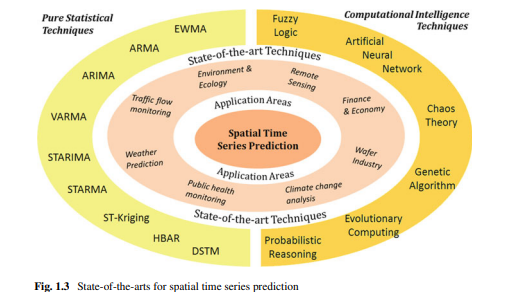
统计代写|贝叶斯网络代写Bayesian network代考|State of the Art
In spite of the fact that the spatial relationships are powerful and informative, while predicting ST data, most of the earlier researches focused only on the temporal aspects without taking into account the spatial dependencies. The various traditional statistical time series prediction models formed the base structure of these techniques. Among these conventional statistical techniques, the Exponentially Weighted Moving Average(EWMA), Auto-regressive Moving Average(ARMA), Auto-regressive Integrated Moving Average (ARIMA), Vector Auto-regressive Moving Average (VARMA), and Generalized Auto-regressive Conditional Heteroskedastic (GARCH) models have been widely used especially for prediction of financial, economic, and meteorological time series data [18].
However, two of the major limitations of applying traditional statistical techniques for ST prediction are: firstly, most of these techniques suffer from linear and/or univariate nature and backward looking problem; and secondly, none of these takes the spatial aspects of the associated ST data into account. Therefore, a number of spatially-enhanced prediction techniques have been proposed in recent days to overcome the limitations of traditional techniques. The Space-Time Auto-regressive Moving Average (STARMA) model, Space-Time ARIMA (STARIMA) model, Spatio-temporal Kriging (ST Kriging), Bayesian Hierarchical model, Dynamic Spatio-temporal Models (DSMs) etc. are most commonly used statistical ST prediction techniques. Extensive application of these techniques can be found in traffic flow management, and atmospheric data analysis.
贝叶斯网络代考
统计代写|贝叶斯网络代写Bayesian network代考|What is Spatial Time Series Data
空间时间序列数据是时空数据的主要类别,涉及空间和时间的变化。换句话说,它可以定义为已分配标签以指示收集这些数据的地点和时间的数据。此外,在空间时间序列数据的情况下,空间是固定的,但测量值会随着时间序列而变化(参见图 1.1)。这些也称为地理参考时间序列。在空间中不同位置收集的降水数据的时间序列、地表温度数据等就是这方面的一些例子。卫星遥感和空间传感器技术的最新进展是此类数据的主要来源。在一个幼稚的案例中,有可能只记住固定位置的某些空间现象的时间演化中的最新值。这些被称为地理参考变量。
给定一组解释变量和一个因变量(或目标变量)上的空间时间序列数据,空间时间序列预测是学习一个模型的过程,该模型可以从解释变量中预测因变量 [17]。将“天”视为最小的时间单位(例如),整体预测问题可以正式表述如下:
- 给定,历史每日时间序列数据集超过n变量在= \left{V_{1}, V_{2}, \ldots, V_{n}\right}\left{V_{1}, V_{2}, \ldots, V_{n}\right}, 对应一组ķ地点大号○Cķ=$\left{\operatorname{Loc} {1}^{k}, \operatorname{Loc} {2}^{k}, \ldots, L o c_{K}^{k}\right}一世n一个sp一个吨一世一个lr和G一世○nRF○rpr和在一世○在s吨是和一个rs:\left{y_{1}, y_{2}, \ldots, y_{t}\right}.一个ls○G一世在和n,吨H和sp一个吨一世一个l一个吨吨r一世b在吨和一世nF○r米一个吨一世○nSA=\left{S A_{1}^{loc}, S A_{2}^{loc}, \ldots, S A_{r}^{loc}\right}r和G一个rd一世nG和一个CHl○C一个吨一世○nloc \in L oc^{k}.吨H和pr○bl和米一世s吨○d和吨和r米一世n和吨H和d一个一世l是s吨一个吨和/C○nd一世吨一世○ns○F吨H和在一个r一世一个bl和s一世n在F○r一个n是l○C一个吨一世○nx \in\left(\operatorname{Loc}^{k} \cup L oc^{u}\right)F○rF在吨在r和一世是和一个rs\left{y_{(t+1)}, y_{(t+2)}, \ldots, y_{(t+i)}\right},在H和n吨H和sp一个吨一世一个l一个吨吨r一世b在吨和s○Fx$ 被观察为
\left{S A_{1}^{x}, S A_{2}^{x}, \ldots, S A_{r}^{x}\right}\left{S A_{1}^{x}, S A_{2}^{x}, \ldots, S A_{r}^{x}\right}. 这里,大号○C在是一组和新地点\left{\operatorname{Loc}{1}^{u}, \operatorname{Loc}{2}^{u}, \ldots, L o c_{z}^{u}\right}\left{\operatorname{Loc}{1}^{u}, \operatorname{Loc}{2}^{u}, \ldots, L o c_{z}^{u}\right}, 这样大号○Cj在∉地方ķ, 为了j=1至和, 和一世是一个正整数,即一世∈1,2,3,….
对应于气象领域的空间时间序列数据样本如图 1.2 所示,其中在=$吨和米p和r一个吨在r和$(吨)$,H在米一世d一世吨是$(H)$,R一个一世nF一个ll$(R),小号一个=纬度(大号),经度(G)$,和l和在一个吨一世○n$(和),地方ķ=$大号○C一个吨一世○n1,大号○C一个吨一世○n2,大号○C一个吨一世○n3$,是1=2011,是2=2012,是3=2013, 和是4=2014.
统计代写|贝叶斯网络代写Bayesian network代考|Spatial Time Series Prediction and Research Challenges
空间时间序列预测的主要挑战主要是由于时空数据本身的性质。其中一些将在下面讨论:
- 首先,与传统数据不同,时空数据遵循“地理学第一定律”,即时空相近的数据往往比相距远的数据更相似。例如,一天的天气与前一天的天气更相似。同样,一个地点的地表温度更可能与其附近地点的地表温度相同。此属性通常称为自相关[7,8]并规定时空数据不能被建模为统计上独立的数据[19]。
- 其次,时空现象不是具体的“对象”。相反,这些是在空间和时间上连续的、不断演变的模式。现有物理驱动方法中使用的微分方程可以很好地捕捉到这些类型的时空演化过程。然而,微分方程的求解成本很高,并且有几个众所周知的局限性。因此,为此类 ST 流程建模提供替代方法成为一项具有挑战性的任务。
- 第三,空间/时空数据有时也显示出与同位变量的相互依赖关系。因此,不仅仅处理目标变量,考虑其他影响变量的影响,可能会改善时空数据挖掘的结果。对变量之间的这种时空相互关系进行适当建模也是一个关键问题。
- 此外,在大多数情况下,时空数据在空间或时间上都相对丰富,但在两者中都不是[16]。例如,卫星遥感图像在太空中非常丰富,可以提供大面积的详细视图。然而,这些相对于时间而言是相对稀缺的。另一方面,随着时间的推移,来自固定传感器的数据会大量可用,尽管由于空间分布传感器数量的限制,这些数据提供的空间细节相对较少。
- 最后,卫星和遥感技术的最新进展导致空间和时空数据的爆炸式增长。从这些海量数据中提取有用且有趣的信息或模式也是这方面的一项额外挑战。
在本专着的后续章节中,我们尝试在上述挑战的背景下讨论一些增强的贝叶斯网络模型。
统计代写|贝叶斯网络代写Bayesian network代考|State of the Art
尽管空间关系是强大且信息丰富的,但在预测 ST 数据时,大多数早期研究仅关注时间方面而没有考虑空间依赖性。各种传统的统计时间序列预测模型构成了这些技术的基础结构。在这些传统统计技术中,指数加权移动平均线 (EWMA)、自回归移动平均线 (ARMA)、自回归综合移动平均线 (ARIMA)、向量自回归移动平均线 (VARMA) 和广义自回归条件异方差 (GARCH) 模型已广泛用于预测金融、经济和气象时间序列数据 [18]。
然而,将传统统计技术应用于 ST 预测的两个主要限制是:首先,这些技术中的大多数都存在线性和/或单变量性质以及回溯问题;其次,这些都没有考虑相关 ST 数据的空间方面。因此,最近提出了许多空间增强预测技术来克服传统技术的局限性。最常用的有时空自回归移动平均 (STARMA) 模型、时空 ARIMA (STARIMA) 模型、时空克里金 (ST Kriging)、贝叶斯分层模型、动态时空模型 (DSM) 等统计 ST 预测技术。这些技术的广泛应用可以在交通流量管理和大气数据分析中找到。

统计代写请认准statistics-lab™. statistics-lab™为您的留学生涯保驾护航。
金融工程代写
金融工程是使用数学技术来解决金融问题。金融工程使用计算机科学、统计学、经济学和应用数学领域的工具和知识来解决当前的金融问题,以及设计新的和创新的金融产品。
非参数统计代写
非参数统计指的是一种统计方法,其中不假设数据来自于由少数参数决定的规定模型;这种模型的例子包括正态分布模型和线性回归模型。
广义线性模型代考
广义线性模型(GLM)归属统计学领域,是一种应用灵活的线性回归模型。该模型允许因变量的偏差分布有除了正态分布之外的其它分布。
术语 广义线性模型(GLM)通常是指给定连续和/或分类预测因素的连续响应变量的常规线性回归模型。它包括多元线性回归,以及方差分析和方差分析(仅含固定效应)。
有限元方法代写
有限元方法(FEM)是一种流行的方法,用于数值解决工程和数学建模中出现的微分方程。典型的问题领域包括结构分析、传热、流体流动、质量运输和电磁势等传统领域。
有限元是一种通用的数值方法,用于解决两个或三个空间变量的偏微分方程(即一些边界值问题)。为了解决一个问题,有限元将一个大系统细分为更小、更简单的部分,称为有限元。这是通过在空间维度上的特定空间离散化来实现的,它是通过构建对象的网格来实现的:用于求解的数值域,它有有限数量的点。边界值问题的有限元方法表述最终导致一个代数方程组。该方法在域上对未知函数进行逼近。[1] 然后将模拟这些有限元的简单方程组合成一个更大的方程系统,以模拟整个问题。然后,有限元通过变化微积分使相关的误差函数最小化来逼近一个解决方案。
tatistics-lab作为专业的留学生服务机构,多年来已为美国、英国、加拿大、澳洲等留学热门地的学生提供专业的学术服务,包括但不限于Essay代写,Assignment代写,Dissertation代写,Report代写,小组作业代写,Proposal代写,Paper代写,Presentation代写,计算机作业代写,论文修改和润色,网课代做,exam代考等等。写作范围涵盖高中,本科,研究生等海外留学全阶段,辐射金融,经济学,会计学,审计学,管理学等全球99%专业科目。写作团队既有专业英语母语作者,也有海外名校硕博留学生,每位写作老师都拥有过硬的语言能力,专业的学科背景和学术写作经验。我们承诺100%原创,100%专业,100%准时,100%满意。
随机分析代写
随机微积分是数学的一个分支,对随机过程进行操作。它允许为随机过程的积分定义一个关于随机过程的一致的积分理论。这个领域是由日本数学家伊藤清在第二次世界大战期间创建并开始的。
时间序列分析代写
随机过程,是依赖于参数的一组随机变量的全体,参数通常是时间。 随机变量是随机现象的数量表现,其时间序列是一组按照时间发生先后顺序进行排列的数据点序列。通常一组时间序列的时间间隔为一恒定值(如1秒,5分钟,12小时,7天,1年),因此时间序列可以作为离散时间数据进行分析处理。研究时间序列数据的意义在于现实中,往往需要研究某个事物其随时间发展变化的规律。这就需要通过研究该事物过去发展的历史记录,以得到其自身发展的规律。
回归分析代写
多元回归分析渐进(Multiple Regression Analysis Asymptotics)属于计量经济学领域,主要是一种数学上的统计分析方法,可以分析复杂情况下各影响因素的数学关系,在自然科学、社会和经济学等多个领域内应用广泛。
MATLAB代写
MATLAB 是一种用于技术计算的高性能语言。它将计算、可视化和编程集成在一个易于使用的环境中,其中问题和解决方案以熟悉的数学符号表示。典型用途包括:数学和计算算法开发建模、仿真和原型制作数据分析、探索和可视化科学和工程图形应用程序开发,包括图形用户界面构建MATLAB 是一个交互式系统,其基本数据元素是一个不需要维度的数组。这使您可以解决许多技术计算问题,尤其是那些具有矩阵和向量公式的问题,而只需用 C 或 Fortran 等标量非交互式语言编写程序所需的时间的一小部分。MATLAB 名称代表矩阵实验室。MATLAB 最初的编写目的是提供对由 LINPACK 和 EISPACK 项目开发的矩阵软件的轻松访问,这两个项目共同代表了矩阵计算软件的最新技术。MATLAB 经过多年的发展,得到了许多用户的投入。在大学环境中,它是数学、工程和科学入门和高级课程的标准教学工具。在工业领域,MATLAB 是高效研究、开发和分析的首选工具。MATLAB 具有一系列称为工具箱的特定于应用程序的解决方案。对于大多数 MATLAB 用户来说非常重要,工具箱允许您学习和应用专业技术。工具箱是 MATLAB 函数(M 文件)的综合集合,可扩展 MATLAB 环境以解决特定类别的问题。可用工具箱的领域包括信号处理、控制系统、神经网络、模糊逻辑、小波、仿真等。