如果你也在 怎样代写贝叶斯网络Bayesian network这个学科遇到相关的难题,请随时右上角联系我们的24/7代写客服。
贝叶斯网络(BN)是一种表示不确定领域知识的概率图形模型,其中每个节点对应一个随机变量,每条边代表相应随机变量的条件概率。
statistics-lab™ 为您的留学生涯保驾护航 在代写贝叶斯网络Bayesian network方面已经树立了自己的口碑, 保证靠谱, 高质且原创的统计Statistics代写服务。我们的专家在代写贝叶斯网络Bayesian network代写方面经验极为丰富,各种代写贝叶斯网络Bayesian network相关的作业也就用不着说。
我们提供的贝叶斯网络Bayesian network及其相关学科的代写,服务范围广, 其中包括但不限于:
- Statistical Inference 统计推断
- Statistical Computing 统计计算
- Advanced Probability Theory 高等概率论
- Advanced Mathematical Statistics 高等数理统计学
- (Generalized) Linear Models 广义线性模型
- Statistical Machine Learning 统计机器学习
- Longitudinal Data Analysis 纵向数据分析
- Foundations of Data Science 数据科学基础
统计代写|贝叶斯网络代写Bayesian network代考|Why SpaBN for Spatial Time Series Prediction
Spatio-temporal variables are not independent. In most of the cases, these are dependent on various other co-located variables. For example, consider a scenario
of predicting water level at a reservoir in the flow of any river. The water level at the reservoir depends on many factors, like the volume of inflow and outflow of water, seepage into ground, evaporation, meteorological condition, and so on. One of the significant meteorological factors in this regard is the environmental precipitation. Now, the level of water in the reservoir depends not only on the precipitation at the reservoir location, but also that in the various other locations in the whole watershed of the corresponding river. Moreover, based on the various topographical factors, like soil type, land cover category, land slope etc., the precipitation at the different locations may have different influence on the water level of the reservoir. Thus, modeling the spatial effect/influence of precipitation or any such meteorological factor on the reservoir water level becomes a challenging issue, inasmuch as the watershed of any river is in general large and consists of locations with varying topographic characteristics.
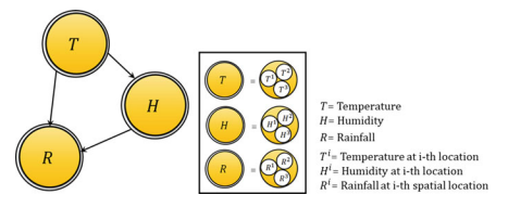
Although the graphical models, like Bayesian networks, are highly suitable for representing such inter-variable influences, yet, for each such influencing variable, introducing representative node corresponding to each spatial location will lead to a very complicated causal dependency graph structure consisting of a large number of nodes and edges. One such example scenario has been illustrated through the Fig. 4.3, which shows a graphical model representing influence from three variables $V_{i}$, $(i=1,2,3)$, distributed at $K=8$ number of spatial locations. This eventually leads to extremely high time and space complexities during parameter learning and inference process. The spatial Bayesian network (SpaBN) can handle this situation efficiently, by using the composite node representation for each spatially distributed variable.
统计代写|贝叶斯网络代写Bayesian network代考|Parameter Learning
Let us assume a directed acyclic graph $G\left(V_{s}, V_{c}, E\right)$, as shown in the Fig. 4.1, where $V_{s}=\left{V_{2}, V_{6}\right}$ denotes the set of standard nodes; $V_{c}=\left{V_{1}, V_{3}, V_{4}, V_{5}\right}$ denotes the set of composite nodes; and $E$ is the set of edges $\left{V_{1} \rightarrow V_{2}, V_{1} \rightarrow\right.$ $\left.V_{3}, \quad V_{1} \rightarrow V_{4}, V_{2} \rightarrow V_{4}, V_{2} \rightarrow V_{5}, V_{3} \rightarrow V_{4}, V_{3} \rightarrow V_{6}, V_{4} \rightarrow V_{5}, V_{4} \rightarrow V_{6}\right}$. An edge from $V_{i}$ to $V_{j}$ can be interpreted as $V_{i}$ has influence on $V_{j}$. Let us also consider that the variables corresponding to the composite nodes are spatially distributed over $K$ ( $=8$ as per the figure) number of locations.
According to the learning principle of SpaBN $[6]$, the marginal probabilities of the composite nodes $\in V_{c}$ in this scenario are calculated with consideration to the spatial importance of each neighboring location:
$$
\begin{aligned}
&\boldsymbol{P}\left(V_{1}\right)=\gamma \cdot\left[\sum_{i=1}^{K} P\left(V_{1}^{i}\right) \cdot S W_{i}\right] \
&P\left(V_{3}\right)=\gamma \cdot\left[\sum_{i=1}^{K} P\left(V_{3}^{i}\right) \cdot S W_{i}\right] \
&P\left(V_{4}\right)=\gamma \cdot\left[\sum_{i=1}^{K} P\left(V_{4}^{i}\right) \cdot S W_{i}\right] \
&P\left(V_{5}\right)=\gamma \cdot\left[\sum_{i=1}^{K} P\left(V_{5}^{i}\right) \cdot S W_{i}\right]
\end{aligned}
$$
where, $\gamma$ is a normalization constant such that the sum of marginal probabilities corresponding to all possible values of the variable becomes $1 . P\left(V_{j}^{i}\right)$ is the marginal probability of singular component $V_{j}^{i}$ in $V_{j}$, for $\mathrm{j}=1,3,4,5$, and $S W_{i}$ is the spatial weight/importance of the $i$ th neighboring location. For example, considering
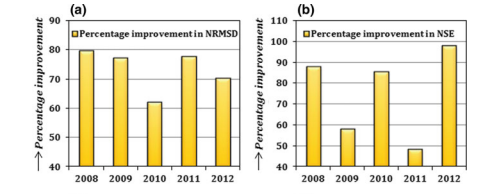
the example scenario in the Chap. 1 (Fig. 1.2) and assuming the prediction location is Location-3, the probability distribution for the variable $T$ for the year 2011 can be estimated as: $P(T 1)=\gamma \cdot\left[\left(T_{1}^{\text {Locl }} \times S W_{L o c 1}\right)+\left(T_{1}^{\text {Loc } 2} \times S W_{L o c 2}\right)+\left(T_{1}^{\text {Loc } 3} \times\right.\right.$ $\left.\left.S W_{\text {Lac3 }}\right)\right]=\gamma \cdot[(0.8 \times 0.03)+(0.0 \times 0.97)+(0.0 \times 1.0)]=0.024 \gamma$. In similar way, we can estimate $P(T 2)=0.006 \gamma, P(T 3)=0.2 \gamma, P(T 4)=1.38 \gamma$, and $P(T 5)=0.39 \gamma$, where $\gamma$ is the normalization constant and can be determined as $0.5$. Thus, the normalized probability distribution for the spatially distributed variable $T$ becomes $P(T 1)=0.012, P(T 2)=0.003, P(T 3)=0.1, P(T 4)=0.69$, $P(T 5)=0.195$
The conditional probabilities, involving composite nodes $\in V_{c}$, are calculated similarly, considering spatial importance of the nearby locations, as follows:
$$
\begin{aligned}
P\left(V_{2} \mid V_{1}\right)=\gamma \cdot & {\left[\sum_{i=1}^{K} \frac{n\left(V_{2}, V_{1}^{i}\right)}{n\left(V_{1}^{i}\right)} \cdot S W_{i}\right] } \
P\left(V_{3} \mid V_{1}\right)=\gamma \cdot & {\left[\sum_{i=1}^{K} \frac{n\left(V_{3}^{i}, V_{1}^{i}\right)}{n\left(V_{1}^{i}\right)} \cdot S W_{i}\right] } \
P\left(V_{4} \mid V_{1}, V_{2}, V_{3}\right)=\gamma \cdot & {\left[\sum_{i=1}^{K} \frac{n\left(V_{1}^{i}, V_{2}, V_{3}^{i}, V_{4}^{i}\right)}{n\left(V_{1}^{i}, V_{2}, V_{3}^{i}\right)} \cdot S W_{i}\right] } \
P\left(V_{5} \mid V_{2}, V_{4}\right)=\gamma \cdot & {\left[\sum_{i=1}^{K} \frac{n\left(V_{5}^{i}, V_{2}, V_{4}^{i}\right)}{n\left(V_{2}, V_{4}^{i}\right)} \cdot S W_{i}\right] } \
P\left(V_{6} \mid V_{3}, V_{4}\right)=\gamma \cdot & {\left[\sum_{i=1}^{K} \frac{n\left(V_{6}, V_{3}^{i}, V_{4}^{i}\right)}{n\left(V_{3}^{i}, V_{4}^{i}\right)}-S W_{i}\right] }
\end{aligned}
$$
where, $n(<,>)$ represents the total number of observation for the variable combination $<\cdot>$. Considering the example scenario presented in Chap. 1 (Fig. 1.2) and assuming the prediction location to be Location-3, the calculation of conditional probability distribution of the variable humidity $(H)$ for the year 2011 are explained through Fig. 4.4, in comparison with standard BN based probability calculation. Here, the structure of SpaBN is considered to be as depicted in Fig. 4.2.
It is to be noted that the causal dependency graph of the SpaBN does not contain any of the spatial attributes (SAs) as described while discussing ST relationship learning in the Chap. 3. Rather, for any variable under study, the network considers relevant node corresponding to each of the associated spatial locations explicitly, and the appropriate spatial attributes are utilized in spatial weight/importance $(S W)$ calculation. The overall process of ST relationship learning using SpaBN is presented through the Algorithm $3 .$
统计代写|贝叶斯网络代写Bayesian network代考|SpaBN-Based Prediction
Once the inferred value is produced, it is further processed to finally generate the predicted value of the variable. Among all the inferred values of the prediction variable, the predicted value becomes the one which is associated with the highest probability estimates $P(\cdot)$. Therefore, if pred $V_{j}$ is the predicted value of the variable $V_{j}$, then $P\left(\operatorname{pred}{V{j}} \mid e\right)=\max \left{P\left(V_{j} \mid e\right)\right}$, where $e$ indicates the given combination of values for the set of evidence variables, and $P\left(V_{j} \mid e\right)$ represents the inferred probability distribution of the variable $V_{j}$ given $e$. With respect to the above example, $P\left(\right.$ pred $\left.V_{6} \mid V_{1}, V_{2}, \ldots, V_{4}\right)=\max \left{P\left(V_{6} \mid V_{1}, V_{2}, \ldots, V_{4}\right)\right}$. Now, since the overall SpaBN analysis is performed considering discretized value of the variables, the predicted value pred ${ }{V j}$ is also obtained in the form of range of values $\left[L B{j}, U B_{j}\right]$. Hence, in order to obtained a single value for the prediction variable, the mid value of the range may be considered. Therefore, finally, $\operatorname{pred}{V{j}}=\left(L B_{j}+U B_{j}\right) / 2$
贝叶斯网络代考
统计代写|贝叶斯网络代写Bayesian network代考|Why SpaBN for Spatial Time Series Prediction
时空变量不是独立的。在大多数情况下,这些取决于各种其他位于同一位置的变量。例如,考虑一个场景
预测任何河流中水库的水位。水库的水位取决于许多因素,如进出水量、渗入地下、蒸发量、气象条件等。这方面的重要气象因素之一是环境降水。现在,水库的水位不仅取决于水库所在地的降水量,还取决于相应河流整个流域内其他各个位置的降水量。此外,根据土壤类型、土地覆被类型、坡度等各种地形因素,不同地点的降水对水库水位的影响可能不同。因此,
尽管像贝叶斯网络这样的图形模型非常适合表示这种变量间的影响,但是,对于每个这样的影响变量,引入与每个空间位置对应的代表节点将导致一个非常复杂的因果依赖图结构,该结构由一个大的节点和边的数量。图 4.3 说明了一个这样的示例场景,该图显示了一个图形模型,表示三个变量的影响在一世, (一世=1,2,3), 分布在ķ=8空间位置的数量。这最终导致参数学习和推理过程中的时间和空间复杂性极高。空间贝叶斯网络 (SpaBN) 可以通过对每个空间分布变量使用复合节点表示来有效地处理这种情况。
统计代写|贝叶斯网络代写Bayesian network代考|Parameter Learning
让我们假设一个有向无环图G(在s,在C,和),如图 4.1 所示,其中V_{s}=\left{V_{2}, V_{6}\right}V_{s}=\left{V_{2}, V_{6}\right}表示标准节点的集合;V_{c}=\left{V_{1}, V_{3}, V_{4}, V_{5}\right}V_{c}=\left{V_{1}, V_{3}, V_{4}, V_{5}\right}表示复合节点的集合;和和是边的集合\left{V_{1} \rightarrow V_{2}, V_{1} \rightarrow\right.$ $\left.V_{3}, \quad V_{1} \rightarrow V_{4}, V_{2} \rightarrow V_{4}, V_{2} \rightarrow V_{5}, V_{3} \rightarrow V_{4}, V_{3} \rightarrow V_{6}, V_{4} \rightarrow V_{5} , V_{4} \rightarrow V_{6}\right}\left{V_{1} \rightarrow V_{2}, V_{1} \rightarrow\right.$ $\left.V_{3}, \quad V_{1} \rightarrow V_{4}, V_{2} \rightarrow V_{4}, V_{2} \rightarrow V_{5}, V_{3} \rightarrow V_{4}, V_{3} \rightarrow V_{6}, V_{4} \rightarrow V_{5} , V_{4} \rightarrow V_{6}\right}. 一个边缘来自在一世至在j可以解释为在一世有影响在j. 让我们还考虑对应于复合节点的变量在空间上分布在ķ ( =8如图)位置的数量。
根据SpaBN的学习原理[6], 复合节点的边际概率∈在C在这种情况下,计算时会考虑每个相邻位置的空间重要性:
磷(在1)=C⋅[∑一世=1ķ磷(在1一世)⋅小号在一世] 磷(在3)=C⋅[∑一世=1ķ磷(在3一世)⋅小号在一世] 磷(在4)=C⋅[∑一世=1ķ磷(在4一世)⋅小号在一世] 磷(在5)=C⋅[∑一世=1ķ磷(在5一世)⋅小号在一世]
在哪里,C是一个归一化常数,使得对应于变量所有可能值的边际概率之和变为1.磷(在j一世)是奇异分量的边际概率在j一世在在j, 为了j=1,3,4,5, 和小号在一世是空间权重/重要性一世th 相邻位置。例如,考虑
章节中的示例场景。1(图 1.2)并假设预测位置是 Location-3,变量的概率分布吨2011 年可估算为:磷(吨1)=C⋅[(吨1本地 ×小号在大号○C1)+(吨1地方 2×小号在大号○C2)+(吨1地方 3× 小号在紫胶3 )]=C⋅[(0.8×0.03)+(0.0×0.97)+(0.0×1.0)]=0.024C. 类似地,我们可以估计磷(吨2)=0.006C,磷(吨3)=0.2C,磷(吨4)=1.38C, 和磷(吨5)=0.39C, 在哪里C是归一化常数,可以确定为0.5. 因此,空间分布变量的归一化概率分布吨变成磷(吨1)=0.012,磷(吨2)=0.003,磷(吨3)=0.1,磷(吨4)=0.69, 磷(吨5)=0.195
条件概率,涉及复合节点∈在C, 计算类似,考虑到附近位置的空间重要性,如下所示:
磷(在2∣在1)=C⋅[∑一世=1ķn(在2,在1一世)n(在1一世)⋅小号在一世] 磷(在3∣在1)=C⋅[∑一世=1ķn(在3一世,在1一世)n(在1一世)⋅小号在一世] 磷(在4∣在1,在2,在3)=C⋅[∑一世=1ķn(在1一世,在2,在3一世,在4一世)n(在1一世,在2,在3一世)⋅小号在一世] 磷(在5∣在2,在4)=C⋅[∑一世=1ķn(在5一世,在2,在4一世)n(在2,在4一世)⋅小号在一世] 磷(在6∣在3,在4)=C⋅[∑一世=1ķn(在6,在3一世,在4一世)n(在3一世,在4一世)−小号在一世]
在哪里,n(<,>)表示变量组合的观察总数<⋅>. 考虑第 1 章中介绍的示例场景。1(图1.2)假设预测位置为Location-3,计算变量湿度的条件概率分布(H)2011 年通过图 4.4 解释,与基于标准 BN 的概率计算进行比较。这里,SpaBN 的结构被认为如图 4.2 所示。
需要注意的是,SpaBN 的因果依赖图不包含任何空间属性(SA),正如在第 1 章中讨论 ST 关系学习时所描述的那样。3. 相反,对于研究中的任何变量,网络明确考虑与每个相关空间位置对应的相关节点,并在空间权重/重要性中使用适当的空间属性(小号在)计算。通过算法呈现使用SpaBN进行ST关系学习的整体过程3.
统计代写|贝叶斯网络代写Bayesian network代考|SpaBN-Based Prediction
一旦产生了推断值,它会被进一步处理以最终生成变量的预测值。在预测变量的所有推断值中,预测值成为与最高概率估计相关联的值磷(⋅). 因此,如果预在j是变量的预测值在j, 然后P\left(\operatorname{pred}{V{j}} \mid e\right)=\max \left{P\left(V_{j} \mid e\right)\right}P\left(\operatorname{pred}{V{j}} \mid e\right)=\max \left{P\left(V_{j} \mid e\right)\right}, 在哪里和表示一组证据变量的给定值组合,并且磷(在j∣和)表示变量的推断概率分布在j给定和. 对于上面的例子,磷(前\left.V_{6} \mid V_{1}, V_{2}, \ldots, V_{4}\right)=\max \left{P\left(V_{6} \mid V_{1}, V_{2}, \ldots, V_{4}\right)\right}\left.V_{6} \mid V_{1}, V_{2}, \ldots, V_{4}\right)=\max \left{P\left(V_{6} \mid V_{1}, V_{2}, \ldots, V_{4}\right)\right}. 现在,由于整体 SpaBN 分析是考虑变量的离散值进行的,因此预测值 pred在j也以取值范围的形式得到[大号乙j,在乙j]. 因此,为了获得预测变量的单个值,可以考虑范围的中间值。因此,最后,前在j=(大号乙j+在乙j)/2

统计代写请认准statistics-lab™. statistics-lab™为您的留学生涯保驾护航。
金融工程代写
金融工程是使用数学技术来解决金融问题。金融工程使用计算机科学、统计学、经济学和应用数学领域的工具和知识来解决当前的金融问题,以及设计新的和创新的金融产品。
非参数统计代写
非参数统计指的是一种统计方法,其中不假设数据来自于由少数参数决定的规定模型;这种模型的例子包括正态分布模型和线性回归模型。
广义线性模型代考
广义线性模型(GLM)归属统计学领域,是一种应用灵活的线性回归模型。该模型允许因变量的偏差分布有除了正态分布之外的其它分布。
术语 广义线性模型(GLM)通常是指给定连续和/或分类预测因素的连续响应变量的常规线性回归模型。它包括多元线性回归,以及方差分析和方差分析(仅含固定效应)。
有限元方法代写
有限元方法(FEM)是一种流行的方法,用于数值解决工程和数学建模中出现的微分方程。典型的问题领域包括结构分析、传热、流体流动、质量运输和电磁势等传统领域。
有限元是一种通用的数值方法,用于解决两个或三个空间变量的偏微分方程(即一些边界值问题)。为了解决一个问题,有限元将一个大系统细分为更小、更简单的部分,称为有限元。这是通过在空间维度上的特定空间离散化来实现的,它是通过构建对象的网格来实现的:用于求解的数值域,它有有限数量的点。边界值问题的有限元方法表述最终导致一个代数方程组。该方法在域上对未知函数进行逼近。[1] 然后将模拟这些有限元的简单方程组合成一个更大的方程系统,以模拟整个问题。然后,有限元通过变化微积分使相关的误差函数最小化来逼近一个解决方案。
tatistics-lab作为专业的留学生服务机构,多年来已为美国、英国、加拿大、澳洲等留学热门地的学生提供专业的学术服务,包括但不限于Essay代写,Assignment代写,Dissertation代写,Report代写,小组作业代写,Proposal代写,Paper代写,Presentation代写,计算机作业代写,论文修改和润色,网课代做,exam代考等等。写作范围涵盖高中,本科,研究生等海外留学全阶段,辐射金融,经济学,会计学,审计学,管理学等全球99%专业科目。写作团队既有专业英语母语作者,也有海外名校硕博留学生,每位写作老师都拥有过硬的语言能力,专业的学科背景和学术写作经验。我们承诺100%原创,100%专业,100%准时,100%满意。
随机分析代写
随机微积分是数学的一个分支,对随机过程进行操作。它允许为随机过程的积分定义一个关于随机过程的一致的积分理论。这个领域是由日本数学家伊藤清在第二次世界大战期间创建并开始的。
时间序列分析代写
随机过程,是依赖于参数的一组随机变量的全体,参数通常是时间。 随机变量是随机现象的数量表现,其时间序列是一组按照时间发生先后顺序进行排列的数据点序列。通常一组时间序列的时间间隔为一恒定值(如1秒,5分钟,12小时,7天,1年),因此时间序列可以作为离散时间数据进行分析处理。研究时间序列数据的意义在于现实中,往往需要研究某个事物其随时间发展变化的规律。这就需要通过研究该事物过去发展的历史记录,以得到其自身发展的规律。
回归分析代写
多元回归分析渐进(Multiple Regression Analysis Asymptotics)属于计量经济学领域,主要是一种数学上的统计分析方法,可以分析复杂情况下各影响因素的数学关系,在自然科学、社会和经济学等多个领域内应用广泛。
MATLAB代写
MATLAB 是一种用于技术计算的高性能语言。它将计算、可视化和编程集成在一个易于使用的环境中,其中问题和解决方案以熟悉的数学符号表示。典型用途包括:数学和计算算法开发建模、仿真和原型制作数据分析、探索和可视化科学和工程图形应用程序开发,包括图形用户界面构建MATLAB 是一个交互式系统,其基本数据元素是一个不需要维度的数组。这使您可以解决许多技术计算问题,尤其是那些具有矩阵和向量公式的问题,而只需用 C 或 Fortran 等标量非交互式语言编写程序所需的时间的一小部分。MATLAB 名称代表矩阵实验室。MATLAB 最初的编写目的是提供对由 LINPACK 和 EISPACK 项目开发的矩阵软件的轻松访问,这两个项目共同代表了矩阵计算软件的最新技术。MATLAB 经过多年的发展,得到了许多用户的投入。在大学环境中,它是数学、工程和科学入门和高级课程的标准教学工具。在工业领域,MATLAB 是高效研究、开发和分析的首选工具。MATLAB 具有一系列称为工具箱的特定于应用程序的解决方案。对于大多数 MATLAB 用户来说非常重要,工具箱允许您学习和应用专业技术。工具箱是 MATLAB 函数(M 文件)的综合集合,可扩展 MATLAB 环境以解决特定类别的问题。可用工具箱的领域包括信号处理、控制系统、神经网络、模糊逻辑、小波、仿真等。