如果你也在 怎样代写金融统计financial statistics这个学科遇到相关的难题,请随时右上角联系我们的24/7代写客服。
金融统计学是研究金融现象数量方面的方法论学科,金融现象是经济现象的一个组成部分。
statistics-lab™ 为您的留学生涯保驾护航 在代写金融统计financial statistics方面已经树立了自己的口碑, 保证靠谱, 高质且原创的统计Statistics代写服务。我们的专家在代写金融统计financial statistics代写方面经验极为丰富,各种代写金融统计financial statistics相关的作业也就用不着说。
我们提供的金融统计financial statistics及其相关学科的代写,服务范围广, 其中包括但不限于:
- Statistical Inference 统计推断
- Statistical Computing 统计计算
- Advanced Probability Theory 高等楖率论
- Advanced Mathematical Statistics 高等数理统计学
- (Generalized) Linear Models 广义线性模型
- Statistical Machine Learning 统计机器学习
- Longitudinal Data Analysis 纵向数据分析
- Foundations of Data Science 数据科学基础
统计代写|金融统计代写financial statistics代考|The Stock Price as a Stochastic Process
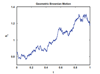
Stock prices are stochastic processes in discrete time which only take discrete values due to the limited measurement scale. Nevertheless, stochastic processes in continuous time are used as models since they are analytically easier to handle than discrete models, e.g. the binomial or trinomial process. However, the latter is more intuitive and proves to be very useful in simulations.
Two features of the general Wiener process $d X_{t}=\mu d t+\sigma d W_{t}$ make it an unsuitable model for stock prices. First, it allows for negative stock prices, and second the local variability is higher for high stock prices. Hence, stock prices $S_{I}$ are modeled by means of the more general Itô-process:
$$
d S_{t}=\mu\left(S_{l}, t\right) d t+\sigma\left(S_{l}, t\right) d W_{l}
$$
This model, however, does depend on the unknown functions $\mu(X, t)$ and $\sigma(X, t)$. A useful and simpler variant utilizing only two unknown real model parameters $\mu$ and $\sigma$ can be justified by the following reflection: The percentage return on the invested capital should on average not depend on the stock price at which the investment is made, and of course, should not depend on the currency unit (EUR, USD,$\ldots$ ) in which the stock price is quoted. Furthermore, the average return should be proportional to the investment horizon, as it is the case for other investment
instruments. Putting things together, we request:
$$
\frac{\mathrm{E}\left[d S_{l}\right]}{S_{l}}=\frac{\mathrm{E}\left[S_{l+d t}-S_{l}\right]}{S_{l}}=\mu \cdot d t
$$
Since $\mathrm{E}\left[d W_{l}\right]=0$ this condition is satisfied if
$$
\mu\left(S_{l}, t\right)=\mu \cdot S_{l}
$$
for given $S_{l}$. Additionally,
$$
\sigma\left(S_{l}, t\right)=\sigma \cdot S_{l}
$$
takes into consideration that the absolute size of the stock price fluctuation is proportional to the currency unit in which the stock price is quoted. In summary, we model the stock price $S_{l}$ as a solution of the stochastic differential equation
$$
d S_{t}=\mu \cdot S_{t} d t+\sigma \cdot S_{t} \cdot d W_{t}
$$
统计代写|金融统计代写financial statistics代考|Itô’s Lemma
A crucial tool in dealing with stochastic differential equations is Itô’s lemma. If $\left{X_{I}, t \geq 0\right}$ is an Itô-process:
$$
d X_{t}=\mu\left(X_{t}, t\right) d t+\sigma\left(X_{t}, t\right) d W_{l},
$$
one is often interested in the dynamics of stochastic processes which are functions of $X_{l}: Y_{t}=g\left(X_{l}\right)$. Then $\left{Y_{l} ; t \geq 0\right}$ can also be described by a solution of a stochastic differential equation from which interesting properties of $Y_{I}$ can be derived, as for example the average growth in time $t$.
For a heuristic derivation of the equation for $\left{Y_{l} ; t \geq 0\right}$ we assume that $g$ is differentiable as many times as necessary. From a Taylor expansion it follows that:
$$
\begin{aligned}
Y_{t+d t}-Y_{l} &=g\left(X_{t+d t}\right)-g\left(X_{t}\right) \
&=g\left(X_{t}+d X_{t}\right)-g\left(X_{t}\right) \
&=\frac{d g}{d X}\left(X_{t}\right) \cdot d X_{t}+\frac{1}{2} \frac{d^{2} g}{d X^{2}}\left(X_{t}\right) \cdot\left(d X_{t}\right)^{2}+\ldots
\end{aligned}
$$
where the dots indicate the terms which can be neglected (for $d t \rightarrow 0$ ). Due to Eq. (5.10) the drift term $\mu\left(X_{t}, t\right) d t$ and the volatility term $\sigma\left(X_{t}, t\right) d W_{t}$ are the dominant terms since for $d t \rightarrow 0$ they are of size $d t$ and $\sqrt{d t}$, respectively.
In doing this, we use the fact that $\mathrm{E}\left[\left(d W_{t}\right)^{2}\right]=d t$ and $d W_{t}=W_{t+d t}-W_{t}$ is of the size of its standard deviation, $\sqrt{d t}$. We neglect terms which are of a smaller size than $d t$. Thus, we can express $\left(d X_{l}\right)^{2}$ by a simpler term:
$$
\begin{aligned}
\left(d X_{t}\right)^{2} &=\left(\mu\left(X_{t}, t\right) d t+\sigma\left(X_{t}, t\right) d W_{t}\right)^{2} \
&=\mu^{2}\left(X_{t}, t\right)(d t)^{2}+2 \mu\left(X_{t}, t\right) \sigma\left(X_{t}, t\right) d t d W_{t}+\sigma^{2}\left(X_{t}, t\right)\left(d W_{t}\right)^{2}
\end{aligned}
$$
We see that the first and the second terms are of size $(d t)^{2}$ and $d t \cdot \sqrt{d t}$, respectively. Therefore, both can be neglected. However, the third term is of size $d t$. More precisely, it can be shown that $d t \rightarrow 0$ :
$$
\left(d W_{l}\right)^{2}=d t
$$
Thanks to this identity, calculus rules for stochastic integrals can be derived from the rules for deterministic functions (as Taylor expansions for example). Neglecting terms which are of smaller size than dt we obtain the following version of Itôs lemma from (5.11):
统计代写|金融统计代写financial statistics代考|Recommended Literature
Exercise 5.1 Let $W_{I}$ be a standard Wiener process. Show that the following processes are also standard Wiener processes:
(a) $X_{t}=c^{-\frac{1}{2}} W_{c l}$ for $c>0$
(b) $Y_{l}=W_{T+l}-W_{T}$ for $T>0$
(c) $V_{t}= \begin{cases}W_{t} & \text { if } t \leq T \ 2 W_{T}-W_{t} & \text { if } t>T\end{cases}$
(d) $Z_{l}=t W_{\frac{1}{l}}$ for $t>0$ and $Z_{l}=0$.
Exercise $5.2$ Calculate $\operatorname{Cov}\left(W_{l}, 3 W_{s}-4 W_{t}\right)$ and $\operatorname{Cov}\left(W_{s}, 3 W_{s}-4 W_{l}\right)$ for $0 \leq s \leq t$.
Exercise $5.3$ Let $W_{t}$ be a standard Wiener process. The process $U_{t}=W_{t}-t W_{1}$ for $t \in[0,1]$ is called Brownian bridge. Calculate its covariance function. What is the distribution of $U_{1}$ ?
Exercise $5.4$ Calculate E $\left(\int_{0}^{2 \pi} W_{s} d W_{s}\right)$
Exercise 5.5 Consider the process $d S_{t}=\mu d t+\sigma d W_{t}$. Find the dynamics of the process $Y_{t}=g\left(S_{l}\right)$, where $g\left(S_{l}, t\right)=2+t+e^{S_{t}}$.
金融统计代写
统计代写|金融统计代写financial statistics代考|The Stock Price as a Stochastic Process
股票价格是离散时间的随机过程,由于测量规模有限,只能取离散值。然而,连续时间的随机过程被用作模型,因为它们在分析上比离散模型更容易处理,例如二项式或三项式过程。然而,后者更直观,并且被证明在模拟中非常有用。
一般维纳过程的两个特征dX吨=μd吨+σd在吨使其成为不适合股票价格的模型。首先,它允许负股票价格,其次,高股票价格的局部可变性更高。因此,股价小号一世通过更一般的伊藤过程建模:
d小号吨=μ(小号l,吨)d吨+σ(小号l,吨)d在l
然而,这个模型确实依赖于未知函数μ(X,吨)和σ(X,吨). 一个有用且更简单的变体,仅使用两个未知的真实模型参数μ和σ可以通过以下反思来证明:投资资本的平均回报率不应取决于进行投资的股票价格,当然也不应取决于货币单位(欧元、美元、…) 报价的股票价格。此外,平均回报应与投资期限成正比,就像其他投资一样
仪器。综上所述,我们要求:
和[d小号l]小号l=和[小号l+d吨−小号l]小号l=μ⋅d吨
自从和[d在l]=0如果满足这个条件
μ(小号l,吨)=μ⋅小号l
给定的小号l. 此外,
σ(小号l,吨)=σ⋅小号l
考虑到股票价格波动的绝对大小与报价的货币单位成正比。总之,我们对股票价格进行建模小号l作为随机微分方程的解
d小号吨=μ⋅小号吨d吨+σ⋅小号吨⋅d在吨
统计代写|金融统计代写financial statistics代考|Itô’s Lemma
处理随机微分方程的一个关键工具是伊藤引理。如果\left{X_{I}, t \geq 0\right}\left{X_{I}, t \geq 0\right}是一个伊藤过程:
dX吨=μ(X吨,吨)d吨+σ(X吨,吨)d在l,
人们通常对随机过程的动力学感兴趣,这些动力学是Xl:是吨=G(Xl). 然后\left{Y_{l} ; t \geq 0\右}\left{Y_{l} ; t \geq 0\右}也可以用一个随机微分方程的解来描述是一世可以推导出来,例如平均时间增长吨.
对于方程的启发式推导\left{Y_{l} ; t \geq 0\右}\left{Y_{l} ; t \geq 0\右}我们假设G可以根据需要多次微分。从泰勒展开可以得出:
是吨+d吨−是l=G(X吨+d吨)−G(X吨) =G(X吨+dX吨)−G(X吨) =dGdX(X吨)⋅dX吨+12d2GdX2(X吨)⋅(dX吨)2+…
其中点表示可以忽略的项(对于d吨→0)。由于方程。(5.10) 漂移项μ(X吨,吨)d吨和波动率项σ(X吨,吨)d在吨是主要术语,因为对于d吨→0它们的大小d吨和d吨, 分别。
在这样做时,我们使用了以下事实和[(d在吨)2]=d吨和d在吨=在吨+d吨−在吨是其标准偏差的大小,d吨. 我们忽略尺寸小于d吨. 因此,我们可以表达(dXl)2用一个更简单的术语:
(dX吨)2=(μ(X吨,吨)d吨+σ(X吨,吨)d在吨)2 =μ2(X吨,吨)(d吨)2+2μ(X吨,吨)σ(X吨,吨)d吨d在吨+σ2(X吨,吨)(d在吨)2
我们看到第一项和第二项是大小(d吨)2和d吨⋅d吨, 分别。因此,两者都可以忽略。但是,第三项是大小d吨. 更准确地说,可以证明d吨→0 :
(d在l)2=d吨
由于这个恒等式,随机积分的微积分规则可以从确定性函数的规则中推导出来(例如泰勒展开式)。忽略比 dt 更小的项,我们从 (5.11) 得到以下版本的 Itôs lemma:
统计代写|金融统计代写financial statistics代考|Recommended Literature
练习 5.1 让在一世是一个标准的维纳过程。证明以下过程也是标准维纳过程:
(a)X吨=C−12在Cl为了C>0
(二)是l=在吨+l−在吨为了吨>0
(C)在吨={在吨 如果 吨≤吨 2在吨−在吨 如果 吨>吨
(d)从l=吨在1l为了吨>0和从l=0.
锻炼5.2计算这(在l,3在s−4在吨)和这(在s,3在s−4在l)为了0≤s≤吨.
锻炼5.3让在吨是一个标准的维纳过程。过程在吨=在吨−吨在1为了吨∈[0,1]被称为布朗桥。计算其协方差函数。什么是分布在1?
锻炼5.4计算 E(∫02圆周率在sd在s)
练习 5.5 考虑过程d小号吨=μd吨+σd在吨. 发现过程的动态是吨=G(小号l), 在哪里G(小号l,吨)=2+吨+和小号吨.

统计代写请认准statistics-lab™. statistics-lab™为您的留学生涯保驾护航。
金融工程代写
金融工程是使用数学技术来解决金融问题。金融工程使用计算机科学、统计学、经济学和应用数学领域的工具和知识来解决当前的金融问题,以及设计新的和创新的金融产品。
非参数统计代写
非参数统计指的是一种统计方法,其中不假设数据来自于由少数参数决定的规定模型;这种模型的例子包括正态分布模型和线性回归模型。
广义线性模型代考
广义线性模型(GLM)归属统计学领域,是一种应用灵活的线性回归模型。该模型允许因变量的偏差分布有除了正态分布之外的其它分布。
术语 广义线性模型(GLM)通常是指给定连续和/或分类预测因素的连续响应变量的常规线性回归模型。它包括多元线性回归,以及方差分析和方差分析(仅含固定效应)。
有限元方法代写
有限元方法(FEM)是一种流行的方法,用于数值解决工程和数学建模中出现的微分方程。典型的问题领域包括结构分析、传热、流体流动、质量运输和电磁势等传统领域。
有限元是一种通用的数值方法,用于解决两个或三个空间变量的偏微分方程(即一些边界值问题)。为了解决一个问题,有限元将一个大系统细分为更小、更简单的部分,称为有限元。这是通过在空间维度上的特定空间离散化来实现的,它是通过构建对象的网格来实现的:用于求解的数值域,它有有限数量的点。边界值问题的有限元方法表述最终导致一个代数方程组。该方法在域上对未知函数进行逼近。[1] 然后将模拟这些有限元的简单方程组合成一个更大的方程系统,以模拟整个问题。然后,有限元通过变化微积分使相关的误差函数最小化来逼近一个解决方案。
tatistics-lab作为专业的留学生服务机构,多年来已为美国、英国、加拿大、澳洲等留学热门地的学生提供专业的学术服务,包括但不限于Essay代写,Assignment代写,Dissertation代写,Report代写,小组作业代写,Proposal代写,Paper代写,Presentation代写,计算机作业代写,论文修改和润色,网课代做,exam代考等等。写作范围涵盖高中,本科,研究生等海外留学全阶段,辐射金融,经济学,会计学,审计学,管理学等全球99%专业科目。写作团队既有专业英语母语作者,也有海外名校硕博留学生,每位写作老师都拥有过硬的语言能力,专业的学科背景和学术写作经验。我们承诺100%原创,100%专业,100%准时,100%满意。
随机分析代写
随机微积分是数学的一个分支,对随机过程进行操作。它允许为随机过程的积分定义一个关于随机过程的一致的积分理论。这个领域是由日本数学家伊藤清在第二次世界大战期间创建并开始的。
时间序列分析代写
随机过程,是依赖于参数的一组随机变量的全体,参数通常是时间。 随机变量是随机现象的数量表现,其时间序列是一组按照时间发生先后顺序进行排列的数据点序列。通常一组时间序列的时间间隔为一恒定值(如1秒,5分钟,12小时,7天,1年),因此时间序列可以作为离散时间数据进行分析处理。研究时间序列数据的意义在于现实中,往往需要研究某个事物其随时间发展变化的规律。这就需要通过研究该事物过去发展的历史记录,以得到其自身发展的规律。
回归分析代写
多元回归分析渐进(Multiple Regression Analysis Asymptotics)属于计量经济学领域,主要是一种数学上的统计分析方法,可以分析复杂情况下各影响因素的数学关系,在自然科学、社会和经济学等多个领域内应用广泛。
MATLAB代写
MATLAB 是一种用于技术计算的高性能语言。它将计算、可视化和编程集成在一个易于使用的环境中,其中问题和解决方案以熟悉的数学符号表示。典型用途包括:数学和计算算法开发建模、仿真和原型制作数据分析、探索和可视化科学和工程图形应用程序开发,包括图形用户界面构建MATLAB 是一个交互式系统,其基本数据元素是一个不需要维度的数组。这使您可以解决许多技术计算问题,尤其是那些具有矩阵和向量公式的问题,而只需用 C 或 Fortran 等标量非交互式语言编写程序所需的时间的一小部分。MATLAB 名称代表矩阵实验室。MATLAB 最初的编写目的是提供对由 LINPACK 和 EISPACK 项目开发的矩阵软件的轻松访问,这两个项目共同代表了矩阵计算软件的最新技术。MATLAB 经过多年的发展,得到了许多用户的投入。在大学环境中,它是数学、工程和科学入门和高级课程的标准教学工具。在工业领域,MATLAB 是高效研究、开发和分析的首选工具。MATLAB 具有一系列称为工具箱的特定于应用程序的解决方案。对于大多数 MATLAB 用户来说非常重要,工具箱允许您学习和应用专业技术。工具箱是 MATLAB 函数(M 文件)的综合集合,可扩展 MATLAB 环境以解决特定类别的问题。可用工具箱的领域包括信号处理、控制系统、神经网络、模糊逻辑、小波、仿真等。