如果你也在 怎样代写金融统计Financial Statistics这个学科遇到相关的难题,请随时右上角联系我们的24/7代写客服。
金融统计是将经济物理学应用于金融市场。它没有采用金融学的规范性根源,而是采用实证主义框架。它包括统计物理学的典范,强调金融市场的突发或集体属性。经验观察到的风格化事实是这种理解金融市场的方法的出发点。
statistics-lab™ 为您的留学生涯保驾护航 在代写金融统计Financial Statistics方面已经树立了自己的口碑, 保证靠谱, 高质且原创的统计Statistics代写服务。我们的专家在代写金融统计Financial Statistics代写方面经验极为丰富,各种代写金融统计Financial Statistics相关的作业也就用不着说。
我们提供的金融统计Financial Statistics及其相关学科的代写,服务范围广, 其中包括但不限于:
- Statistical Inference 统计推断
- Statistical Computing 统计计算
- Advanced Probability Theory 高等概率论
- Advanced Mathematical Statistics 高等数理统计学
- (Generalized) Linear Models 广义线性模型
- Statistical Machine Learning 统计机器学习
- Longitudinal Data Analysis 纵向数据分析
- Foundations of Data Science 数据科学基础
统计代写|金融统计代写Financial Statistics代考|Applications
8.1. Inference on the Gold Price Data (In US Dollars) (1980-2013)
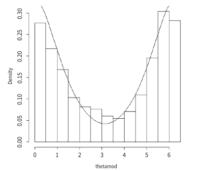
Gold price data, say $x_{t}$, were collected per ounce in US dollars over the years $1980-2013 .$ These were transformed as $z_{t}=100\left(\ln \left(x_{t}\right)-\ln \left(x_{t-1}\right)\right)$, which were then “wrapped” to obtain $\theta_{t}=z_{t} \bmod 2 \pi$ and finally transformed to $\hat{\theta}=\left(\theta_{t}-\bar{\theta}\right) \bmod 2 \pi$, where $\bar{\theta}$ denotes the mean direction of $\theta_{t}$ and $\hat{\theta}$ denotes the variable thetamod as used in the graphs. The Durbin-Watson test performed on the log ratio transformed data shows that the autocorrelation is zero. The test statistic of Watson’s goodness of fit Jammalamadaka and SenGupta (2001) for wrapped stable distribution was obtained as $0.01632691$ and the corresponding P-value was obtained as $0.9970284$, which is greater than $0.05$, indicating that the wrapped stable distribution fits the transformed gold price data (in US dollars). The modified truncated estimate $\hat{\alpha}_{1}^{*}$ is $0.3752206$ while the estimate by characteristic function method is $0.401409$. The value of the objective function using the characteristic function estimate is $2.218941$ while that using our modified truncated estimate is $2.411018$.
8.2. Inference on the Silver Price Data (In US Dollars) (1980-2013)
Data on the price of silver in US dollars collected per ounce over the same time period also underwent the same transformation. The Durbin-Watson test performed on the log ratio transformed data shows that the autocorrelation is zero. Here, the Watson’s goodness of fit test for wrapped stable distribution was also performed and the value of the statistic was obtained as $0.02530653$ and the corresponding $p$-value is $0.9639666$, which is greater than $0.05$, indicating that the wrapped stable distribution also fits the transformed silver price data (in US dollars). The modified truncated estimate of the index parameter $\alpha$ is $0.4112475$ while the estimate by characteristic function method is $0.644846 .$ The value of the objective function using the characteristic function estimate is $2.234203$ while that using our modified truncated estimate is $2.234432$.
统计代写|金融统计代写Financial Statistics代考|Findings and Concluding Remarks
It can be observed from Table 1 that the asymptotic variance of the untruncated estimator is reduced for the corresponding truncated estimator, indicating the efficiency of the truncated estimator.
It can also be noted from Table 2 that, for $\alpha=1.01$, the RMSE of the modified truncated estimator is less than that of the Hill estimator when the sample is relocated by three different relocations, viz. true mean $=0$, sample mean, and sample median, for higher values of the concentration parameter $\rho=0.5,0.6,0.8$, and $0.9$ for sample sizes $n=100,250,500$, and 1000 and for $\rho=0.3,0.4,0.6,0.8$, and $0.9$ for sample sizes $n=2000,5000$, and 10,000 . Furthermore, it can be observed that, for $\alpha=1.25,1.5$, $1.75$ and 1.9, the RMSE of the modified truncated is less than that of the Hill estimator for different relocations for $\rho=0.6,0.7,0.8$, and $0.9$ for smaller sample size and even for $\rho=0.5$ for larger sample size. This clearly indicates the efficiency of the modified truncated estimator over the Hill estimator for higher values of the concentration parameter $\rho$.
It can be observed in Table 3 that the RMSE of the modified truncated estimator is less than that of the characteristic function-based estimator for almost all values of $\alpha$ corresponding to all values of $\sigma$.
The Hill estimator (Dufour and Kurz-Kim $(2010)$ ) is defined for $1 \leq \alpha \leq 2$, whereas the modified truncated estimator is defined for the whole range $0 \leq \alpha \leq 2$. In addition, the overall performance of the modified truncated estimator is quite good in terms of efficiency and consistency over both the Hill estimator and the characteristic function-based estimator.
Thus, we have established an estimator of the index parameter $\alpha$ that strongly supports its parameter space $(0,2]$. It can be observed from the above real life data applications that the modified truncated estimator is quite close to that of the characteristic function-based estimator. In addition, it is simpler and computationally easier than that of the estimator defined in Anderson and Arnold (1993). Thus, it may be considered as a better estimator.
Again, when the estimator of $a$ lies between 1 and 2 , is attempted to model a mixture of two distributions with the value of the index parameter as that of the two extreme tails that is modeling a mixture of Cauchy $(\alpha=1)$ and normal $(\alpha=2)$ distributions when $1<\alpha<2$ or modeling a mixture of Double Exponential $\left(\alpha=\frac{1}{2}\right)$ and Cauchy $(\alpha=1)$ distributions when $\frac{1}{2}<\alpha<1$. Then, it is compared with that of the stable family of distributions for goodness of fit.
We could have used the usual technique of non-linear optimization as used in Salimi et al. (2018) for estimation, but it is computationally demanding and also the (statistical) consistency of the estimators obtained by such method is unknown. In contrast, our proposed methods of trigonometric moment and modified truncated estimation are much simpler, computationally easier and also possess useful consistency properties and, even their asymptotic distributions can be presented in simple and elegant forms as already proved above.
统计代写|金融统计代写Financial Statistics代考|Background
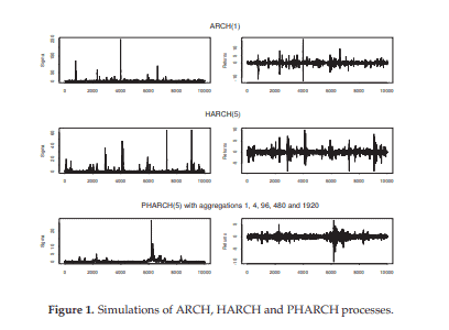
In this section we provide briefly some background on Markov chains and results on stationarity of PHARCH models.
2.1. Markoo Chains
Suppose that $\mathbf{X}=\left{X_{n}, n \in \mathbb{Z}^{+}\right}, \mathbb{Z}^{+}:={0,1,2, \ldots}$ are random variables defined over $(\Omega, \mathcal{F}, \mathcal{B}(\Omega))$, and assume that $\mathrm{X}$ is a Markov chain with transition probability $P(x, A), x \in \Omega, A \subset \Omega$. Then we have the following definitions:
- A function $f: \Omega \rightarrow \mathbb{R}$ is called the smallect semi-continuous function if $\liminf _{y \rightarrow x} f(y) \geq$ $f(x), x \in \Omega$. If $P(\cdot, A)$ is the smallest semi-continuous function for any open set $A \in \mathcal{B}(\Omega)$, we say that (the chain) $\mathbf{X}$ is a weak Feller chain.
- A chain $\mathbf{X}$ is called $\varphi$-irreducible if there exists a measure $\varphi$ on $\mathcal{B}(\Omega)$ such that, for all $x$, whenever $\varphi(A)>0$, we have,
$$
U(x, A)=\sum_{n=1}^{\infty} P^{n}(x, A)>0 .
$$ - The measure $\psi$ is called maximal with respect to $\varphi$, and we write $\psi>\varphi$, if $\psi(A)=0$ implies $\varphi(A)=0$, for all $A \in \mathcal{B}(\Omega)$. If $\mathbf{X}$ is $\varphi$-irreducible, then there exists a probability measure $\psi$, maximal, such that $\mathbf{X}$ is $\psi$-irreducible.
- Let $d={d(n)}$ a distribution or a probability measure on $\mathbb{Z}^{+}$, and consider the Markov chain $\mathbf{X}{d}$ with transition kernel $$ K{d}(x, A):=\sum_{n=0}^{\infty} P^{n}(x, A) d(n)
$$
If there exits a transition kernel $T$ satisfying
$$
K_{d}(x, A) \geq T(x, A), \quad x \in \Omega, A \in \mathcal{B}(\Omega),
$$
then $T$ is called the continuous component of $K_{d}$. - If $\mathbf{X}$ is a Markov chain for which there exits a (sample) distribution $d$ such that $K_{d}$ has a continuous component $T$, with $T(x, \Omega)>0, \forall x$, then $\mathbf{X}$ is called a $T$-chain.
- A measure $\pi$ over $\mathcal{B}(\Omega), \sigma$-finite, with the property
$$
\pi(A)=\int_{\Omega} \pi(d x) P(x, A), A \in \mathcal{B}(\Omega)
$$
is called an invariant measure.
The following two lemmas will be useful. See Meyn and Tweedie (1996) for the proofs and further details. We denote by $I_{A}(\cdot)$ the indicator function of $A$.
金融统计代考
统计代写|金融统计代写Financial Statistics代考|Applications
8.1。黄金价格数据推断(以美元计)(1980-2013)
黄金价格数据,比如X吨, 多年来按每盎司美元收集1980−2013.这些被转换为和吨=100(ln(X吨)−ln(X吨−1)),然后将其“包装”以获得θ吨=和吨反对2圆周率最后转变为θ^=(θ吨−θ¯)反对2圆周率, 在哪里θ¯表示平均方向θ吨和θ^表示图中使用的变量 thetamod。对对数比转换数据执行的 Durbin-Watson 检验表明自相关为零。沃森拟合优度 Jammalamadaka 和 SenGupta (2001) 对包裹稳定分布的检验统计量为0.01632691并获得相应的 P 值0.9970284, 大于0.05,表明包裹的稳定分布拟合转换后的黄金价格数据(以美元计)。修改后的截断估计一个^1∗是0.3752206而特征函数法的估计是0.401409. 使用特征函数估计的目标函数值为2.218941而使用我们修改后的截断估计是2.411018.
8.2. 白银价格数据推论(以美元计)(1980-2013)
同一时期每盎司收集的以美元计的白银价格数据也经历了同样的转变。对对数比转换数据执行的 Durbin-Watson 检验表明自相关为零。在这里,还进行了包裹稳定分布的 Watson 拟合优度检验,得到的统计量值为0.02530653和相应的p-值是0.9639666, 大于0.05,表明包裹的稳定分布也符合转换后的白银价格数据(以美元计)。指数参数的修正截断估计一个是0.4112475而特征函数法的估计是0.644846.使用特征函数估计的目标函数值为2.234203而使用我们修改后的截断估计是2.234432.
统计代写|金融统计代写Financial Statistics代考|Findings and Concluding Remarks
从表1可以看出,对于相应的截断估计量,未截断估计量的渐近方差减小,表明截断估计量的效率。
从表 2 还可以看出,对于一个=1.01,当样本被三个不同的重定位,即。真正的意思=0、样本均值和样本中位数,用于更高的浓度参数值ρ=0.5,0.6,0.8, 和0.9样本量n=100,250,500, 和 1000 和ρ=0.3,0.4,0.6,0.8, 和0.9样本量n=2000,5000, 和 10,000 。此外,可以观察到,对于一个=1.25,1.5, 1.75和 1.9,修改截断的 RMSE 小于 Hill 估计的不同重定位ρ=0.6,0.7,0.8, 和0.9对于较小的样本量,甚至对于ρ=0.5对于更大的样本量。这清楚地表明了改进的截断估计器在 Hill 估计器上的效率,用于更高的浓度参数值ρ.
在表 3 中可以观察到,对于几乎所有一个对应于的所有值σ.
Hill 估计器(Dufour 和 Kurz-Kim(2010)) 定义为1≤一个≤2,而修改的截断估计量是为整个范围定义的0≤一个≤2. 此外,改进的截断估计器的整体性能在效率和一致性方面都优于希尔估计器和基于特征函数的估计器。
因此,我们建立了指数参数的估计量一个强烈支持其参数空间(0,2]. 从上述现实生活中的数据应用中可以看出,修改后的截断估计器与基于特征函数的估计器非常接近。此外,它比 Anderson 和 Arnold (1993) 中定义的估计器更简单,计算更容易。因此,它可以被认为是一个更好的估计量。
同样,当一个介于 1 和 2 之间,试图用索引参数的值对两个分布的混合进行建模,作为对柯西混合建模的两个极端尾部的值(一个=1)和正常的(一个=2)分布时1<一个<2或模拟双指数的混合(一个=12)和柯西(一个=1)分布时12<一个<1. 然后,将其与稳定分布族的拟合优度进行比较。
我们可以使用 Salimi 等人使用的常用非线性优化技术。(2018)用于估计,但它对计算的要求很高,而且通过这种方法获得的估计量的(统计)一致性也是未知的。相比之下,我们提出的三角矩和改进的截断估计方法更简单,计算更容易,并且还具有有用的一致性属性,甚至它们的渐近分布也可以以简单和优雅的形式呈现,如上面已经证明的那样。
统计代写|金融统计代写Financial Statistics代考|Background
在本节中,我们简要介绍马尔可夫链的一些背景以及 PHARCH 模型平稳性的结果。
2.1。Markoo 链
假设\mathbf{X}=\left{X_{n}, n \in \mathbb{Z}^{+}\right}, \mathbb{Z}^{+}:={0,1,2, \ldots }\mathbf{X}=\left{X_{n}, n \in \mathbb{Z}^{+}\right}, \mathbb{Z}^{+}:={0,1,2, \ldots }是定义的随机变量(Ω,F,乙(Ω)),并假设X是具有转移概率的马尔可夫链磷(X,一个),X∈Ω,一个⊂Ω. 那么我们有以下定义:
- 一个函数F:Ω→R称为 smallect 半连续函数,如果林信息是→XF(是)≥ F(X),X∈Ω. 如果磷(⋅,一个)是任何开集的最小半连续函数一个∈乙(Ω),我们说(链)X是一个弱 Feller 链。
- 一条链子X叫做披-如果存在测度则不可约披上乙(Ω)这样,对于所有人X, 每当披(一个)>0, 我们有,
在(X,一个)=∑n=1∞磷n(X,一个)>0. - 的措施ψ被称为最大关于披,我们写ψ>披, 如果ψ(一个)=0暗示披(一个)=0, 对所有人一个∈乙(Ω). 如果X是披- 不可约,则存在概率测度ψ, 最大, 这样X是ψ- 不可约。
- 让d=d(n)分布或概率测度从+,并考虑马尔可夫链Xd带有转换内核ķd(X,一个):=∑n=0∞磷n(X,一个)d(n)
如果存在过渡内核吨令人满意的
ķd(X,一个)≥吨(X,一个),X∈Ω,一个∈乙(Ω),
然后吨称为连续分量ķd. - 如果X是一个存在(样本)分布的马尔可夫链d这样ķd有一个连续的分量吨, 和吨(X,Ω)>0,∀X, 然后X被称为吨-链。
- 一种方法圆周率超过乙(Ω),σ- 有限的,与财产
圆周率(一个)=∫Ω圆周率(dX)磷(X,一个),一个∈乙(Ω)
称为不变测度。
以下两个引理将很有用。有关证明和更多详细信息,请参见 Meyn 和 Tweedie (1996)。我们表示我一个(⋅)的指标函数一个.

统计代写请认准statistics-lab™. statistics-lab™为您的留学生涯保驾护航。
金融工程代写
金融工程是使用数学技术来解决金融问题。金融工程使用计算机科学、统计学、经济学和应用数学领域的工具和知识来解决当前的金融问题,以及设计新的和创新的金融产品。
非参数统计代写
非参数统计指的是一种统计方法,其中不假设数据来自于由少数参数决定的规定模型;这种模型的例子包括正态分布模型和线性回归模型。
广义线性模型代考
广义线性模型(GLM)归属统计学领域,是一种应用灵活的线性回归模型。该模型允许因变量的偏差分布有除了正态分布之外的其它分布。
术语 广义线性模型(GLM)通常是指给定连续和/或分类预测因素的连续响应变量的常规线性回归模型。它包括多元线性回归,以及方差分析和方差分析(仅含固定效应)。
有限元方法代写
有限元方法(FEM)是一种流行的方法,用于数值解决工程和数学建模中出现的微分方程。典型的问题领域包括结构分析、传热、流体流动、质量运输和电磁势等传统领域。
有限元是一种通用的数值方法,用于解决两个或三个空间变量的偏微分方程(即一些边界值问题)。为了解决一个问题,有限元将一个大系统细分为更小、更简单的部分,称为有限元。这是通过在空间维度上的特定空间离散化来实现的,它是通过构建对象的网格来实现的:用于求解的数值域,它有有限数量的点。边界值问题的有限元方法表述最终导致一个代数方程组。该方法在域上对未知函数进行逼近。[1] 然后将模拟这些有限元的简单方程组合成一个更大的方程系统,以模拟整个问题。然后,有限元通过变化微积分使相关的误差函数最小化来逼近一个解决方案。
tatistics-lab作为专业的留学生服务机构,多年来已为美国、英国、加拿大、澳洲等留学热门地的学生提供专业的学术服务,包括但不限于Essay代写,Assignment代写,Dissertation代写,Report代写,小组作业代写,Proposal代写,Paper代写,Presentation代写,计算机作业代写,论文修改和润色,网课代做,exam代考等等。写作范围涵盖高中,本科,研究生等海外留学全阶段,辐射金融,经济学,会计学,审计学,管理学等全球99%专业科目。写作团队既有专业英语母语作者,也有海外名校硕博留学生,每位写作老师都拥有过硬的语言能力,专业的学科背景和学术写作经验。我们承诺100%原创,100%专业,100%准时,100%满意。
随机分析代写
随机微积分是数学的一个分支,对随机过程进行操作。它允许为随机过程的积分定义一个关于随机过程的一致的积分理论。这个领域是由日本数学家伊藤清在第二次世界大战期间创建并开始的。
时间序列分析代写
随机过程,是依赖于参数的一组随机变量的全体,参数通常是时间。 随机变量是随机现象的数量表现,其时间序列是一组按照时间发生先后顺序进行排列的数据点序列。通常一组时间序列的时间间隔为一恒定值(如1秒,5分钟,12小时,7天,1年),因此时间序列可以作为离散时间数据进行分析处理。研究时间序列数据的意义在于现实中,往往需要研究某个事物其随时间发展变化的规律。这就需要通过研究该事物过去发展的历史记录,以得到其自身发展的规律。
回归分析代写
多元回归分析渐进(Multiple Regression Analysis Asymptotics)属于计量经济学领域,主要是一种数学上的统计分析方法,可以分析复杂情况下各影响因素的数学关系,在自然科学、社会和经济学等多个领域内应用广泛。
MATLAB代写
MATLAB 是一种用于技术计算的高性能语言。它将计算、可视化和编程集成在一个易于使用的环境中,其中问题和解决方案以熟悉的数学符号表示。典型用途包括:数学和计算算法开发建模、仿真和原型制作数据分析、探索和可视化科学和工程图形应用程序开发,包括图形用户界面构建MATLAB 是一个交互式系统,其基本数据元素是一个不需要维度的数组。这使您可以解决许多技术计算问题,尤其是那些具有矩阵和向量公式的问题,而只需用 C 或 Fortran 等标量非交互式语言编写程序所需的时间的一小部分。MATLAB 名称代表矩阵实验室。MATLAB 最初的编写目的是提供对由 LINPACK 和 EISPACK 项目开发的矩阵软件的轻松访问,这两个项目共同代表了矩阵计算软件的最新技术。MATLAB 经过多年的发展,得到了许多用户的投入。在大学环境中,它是数学、工程和科学入门和高级课程的标准教学工具。在工业领域,MATLAB 是高效研究、开发和分析的首选工具。MATLAB 具有一系列称为工具箱的特定于应用程序的解决方案。对于大多数 MATLAB 用户来说非常重要,工具箱允许您学习和应用专业技术。工具箱是 MATLAB 函数(M 文件)的综合集合,可扩展 MATLAB 环境以解决特定类别的问题。可用工具箱的领域包括信号处理、控制系统、神经网络、模糊逻辑、小波、仿真等。