如果你也在 怎样代写随机过程stochastic process这个学科遇到相关的难题,请随时右上角联系我们的24/7代写客服。
随机过程被定义为随机变量X={Xt:t∈T}的集合,定义在一个共同的概率空间上,在一个共同的集合S(状态空间)中取值,并以一个集合T为索引,通常是N或[0,∞],并被认为是时间(分别为离散或连续)。
statistics-lab™ 为您的留学生涯保驾护航 在代写随机过程stochastic process方面已经树立了自己的口碑, 保证靠谱, 高质且原创的统计Statistics代写服务。我们的专家在代写随机过程stochastic process代写方面经验极为丰富,各种代写随机过程stochastic process相关的作业也就用不着说。
我们提供的随机过程stochastic process及其相关学科的代写,服务范围广, 其中包括但不限于:
- Statistical Inference 统计推断
- Statistical Computing 统计计算
- Advanced Probability Theory 高等概率论
- Advanced Mathematical Statistics 高等数理统计学
- (Generalized) Linear Models 广义线性模型
- Statistical Machine Learning 统计机器学习
- Longitudinal Data Analysis 纵向数据分析
- Foundations of Data Science 数据科学基础
统计代写|随机过程代写stochastic process代考|For the data set on significant
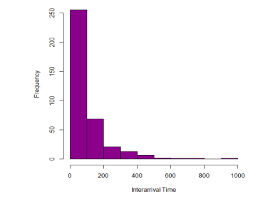
EXERCISE 3.7. For the data set on significant volcanic eruptions between 1920 and 2020 , the code below calculates interarrival times, plots a histogram, and conducts the goodness-of-fit test. The pvalue for the test is larger than $0.05$, indicating that the Poisson process models the data well.
volcanoes. data<- read.csv(file=”. /volcanoesdata.csv”, header=TRUE, sep=”, “)
creating date-time variable
datetime<- as.POSIXct (paste (as. Date (volcanoes. dataSDATE), volcanoes. data\$TIME))
computing lag
datetime. ag $<-$ c $(0$, head (datetime, $-1))$
volcanoes. data<- read.csv (file=”,/volcanoesdata.csv”, header=TRUE, sep=”, “)
creating date-time variable
datetime<- as.POSIXct (paste(as. Date (volcanoes. data\$DATE), volcanoes. data\$TIME))
computing lag
datetime. lag<- c (0, head (datetime, -1))
computing interarrival times (in hours)
int<- (as. numeric(datetime)-as. numeric(datetime. lag))/(3600*24)
int<- int [-1] # removing first value
plotting histogram
hist (int, main=”n, xlab=”Interarrival Time”, col=”dark magenta”)
computing interarrival times (in hours)
int<- (as. numeric (datetime)-as. numeric(datetime. $1 \mathrm{ag})) /(3600 * 24$ )
int<- int[-1] # removing first value
plotting histogram
hist(int, main=”n, xlab=” Interarrival Time”, col=”dark magenta”)
binning interarrival times
binned.int<- as. factor (ifelse (int<25, “1”, ifelse (int>=25 \& int<50, “2”, ifelse (int>=50 \& int<100, “3”, ifelse (int>=100 \& int<150, “4”, ifelse (int>=150 \&
int<200, “5”, ifelse(int>=200 \& int<250, ${ }^{} 6^{}$, ” $\left.\left.\left.\left.\left.\left.7^{*}\right)\right)\right)\right\rangle\right)\right)$
computing observed frequencies
obs<- table (binned. int)
estimating mean for exponential distribution
mean.est<- mean (int)
computing expected frequencies
$\exp <-c(1: 7)$
$\exp [1]<-$ length $(i n t) (1-\exp (-25 /$ mean, $\operatorname{est}))$ $\exp [2]<-$ length (int) $(\exp (-25 /$ mean.est) $-\exp (-50 / \mathrm{mean}$. est) )
$\exp [3]<-$ length (int) * (exp $(-50 /$ mean.est) $-\exp (-100 / \mathrm{mean}$. est $))$
$\exp [4]<-$ length (int) $(\exp (-100 /$ mean .est) $-\exp (-150 / \mathrm{mean}$. est) ) $\exp [5]<-$ length (int) $(\exp (-150 /$ mean.est $)-\exp (-200 /$ mean.est) $)$
统计代写|随机过程代写stochastic process代考|The number of broken
EXERCISE 4.1. (a) The number of broken calculators can be modeled according to a nonhomogeneous Poisson process ${N(t), t \geq 0}$ with the intensity rate function
$$
\lambda(t)=\left{\begin{array}{cc}
3, & \text { if } 0 \leq t \leq 3, \
2 t-3, & \text { if } 3 \leq t \leq 10
\end{array}\right.
$$
The integrated rate function is
$$
\Lambda(t)=\int_{0}^{t} \lambda(u) d u= \begin{cases}\int_{0}^{t} 3 d u=3 t, & \text { if } 0 \leq t \leq 3 \ 9+\int_{3}^{t}(2 u-3) d u=t^{2}-3 t+9, & \text { if } \quad 3 \leq t \leq 10\end{cases}
$$
The probability mass function is
$$
P(N(t)-N(s)=n)=\frac{(\Lambda(t)-\Lambda(s))^{n}}{n !} e^{-(\Lambda(t)-\Lambda(s))}=\frac{\left(t^{2}-s^{2}-3(t-s)\right)^{n}}{n !} e^{-\left(t^{2}-s^{2}-3(t-s)\right)}
$$
(b) $P(N(8)-N(4)=50)=\frac{\left(8^{2}-4^{2}-3(8-4)\right)^{50}}{50 !} e^{-\left(8^{2}-4^{2}-3(8-4)\right)}=0.004983$.
(c) $E(N(10)-N(2))=\Lambda(10)-\Lambda(2)=10^{2}-(3)(10)+9-(3)(2)=73$.
EXERCISE 4.2. (a) Below is the R code and plot of the intensity function $\lambda(t)=-0.000025 t^{3}+$ $0.002 t^{2}+0.12 t$ against $t$ on the interval $[0,120]$.
lambda<- function (t) $-0.000025^{*} t^{\wedge} 3+0.002 *^{\wedge} t^{\wedge} 2+0.12 * t$
lambda<- function (t) $-0.0000$ $t<-\operatorname{seq}(0,120$, by $=0.01)$
$t<-\operatorname{seq}(0,120$, by
统计代写|随机过程代写stochastic process代考|The intensity function looks
The intensity function looks like a skewed upside-down parabola that is equal to 0 at $t=0$ and $t=$ 120 . It achieves the maximum at time $t$ that solves the equation $\lambda^{\prime}(t)=0$. Therefore, $t$ solves the quadratic equation $(-0.000025)(3) t^{2}+(0.002)(2) t+0.12=0$, which simplifies to $-0.0075 t^{2}+$ $0.4 t+12=0$. We need the solution that lies between 0 and 120 , therefore, $t=\frac{0.4+\sqrt{0.52}}{0.015}=$
$74.74068$ days. Thus the peak intensity rate occurs $74.74$ days into the fire season, and the maximum number of fires per day is $=-0.000025(74.74068)^{3}+0.002(74.74068)^{2}+0.12(74.74068)=$ $9.703286$, or roughly $9.7$ fires per day.
(b) We write $\Lambda(t)=\int_{0}^{t} \lambda(u) d u=\int_{0}^{t}\left(-0.000025 u^{3}+0.002 u^{2}+0.12 u\right) d u=-0.00000625 t^{4}+$ $0.0006667 t^{3}+0.06 t^{2}, 0 \leq t \leq 120$. The R code and the graph are given below.
Lambda<- function (t) $-0.00000625 * t^{\wedge} 4+0.0006667^{*} t^{\wedge} 3+0.06 * t^{\wedge} 2$
Lambda<- function (t) $-0.0000$ $t<-$ seq $(0,120$, by $=0.01)$
plot(t, Lambda (t))
To find the average number of wildfires per season we compute $\Lambda(120)=-(0.00000625)(120)^{4}+$ $(0.0006667)(120)^{3}+(0.06)(120)^{2}=720.0576$, so, on average, about 720 fires occur in this area every season.
(a) The middle $50 \%$ of the fire season falls between day 30 and day 90 . The mean number of wildfires in this period is $\Lambda(90)-\Lambda(30)=-(0.00000625)(90)^{4}+(0.0006667)(90)^{3}+(0.06)(90)^{2}-$ $\left(-(0.00000625)(30)^{4}+(0.0006667)(30)^{3}+(0.06)(30)^{2}\right)=561.9618-66.9384=495.0234 .$
随机过程代写
统计代写|随机过程代写stochastic process代考|For the data set on significant
练习 3.7。对于 1920 年至 2020 年间重大火山爆发的数据集,下面的代码计算到达间隔时间,绘制直方图,并进行拟合优度检验。测试的 pvalue 大于0.05,表明泊松过程很好地对数据进行了建模。
火山。数据<- read.csv(file=”./volcanoesdata.csv”, header=TRUE, sep=”, “)
创建日期时间变量
datetime<- as.POSIXct (粘贴(as.Date (volcanoes.dataSDATE),volcanes.data $ TIME))
计算滞后
约会时间。银<−C(0, 头 (日期时间,−1))
火山。数据<- read.csv (file=”,/volcanoesdata.csv”, header=TRUE, sep=”, “)
创建日期时间变量
datetime<- as.POSIXct (paste(as.Date (volcanoes.data $ DATE), volcanes.data $ TIME))
计算滞后
约会时间。滞后<- c (0, head (datetime, -1))
计算到达间隔时间(以小时为单位)
int<- (as. numeric(datetime)-as. numeric(datetime.lag))/(3600*24)
int<- int [-1] # 删除第一个值
绘制直方图
hist (int, main=”n, xlab=”Interarrival Time”, col=”dark magenta”)
计算到达间隔时间(以小时为单位)
int<- (as. numeric (datetime)-as. numeric(datetime.1一种G))/(3600∗24)
int<- int[-1] # 删除第一个值
绘制直方图
hist(int, main=”n, xlab=” 到达间隔时间”, col=”深洋红色”)
分箱间隔时间
binned.int<- 作为。因子 (ifelse (int<25, “1”, ifelse (int>=25 \& int<50, “2”, ifelse (int>=50 \& int<100, “3”, ifelse (int>=100 \& int<150, “4”, ifelse (int>=150 \&
int<200, “5”, ifelse(int>=200 \& int<250, ${ }^{ } 6^{ },”\left.\left.\left.\left.\left.\left.7^{*}\right)\right)\right)\right\rangle\right)\right)$
计算观察到的频率
obs<- 表(binned.int)
估计指数分布的均值
mean.est<- mean (int)
计算预期频率
经验<−C(1:7)
经验[1]<−长度(一世n吨)(1−经验(−25/意思是,是)) 经验[2]<−长度(整数)(经验(−25/平均数)−经验(−50/米和一种n. 是) )
经验[3]<−长度 (int) * (exp(−50/平均数)−经验(−100/米和一种n. 是))
经验[4]<−长度(整数)(经验(−100/平均.est)−经验(−150/米和一种n. 是) )经验[5]<−长度(整数)(经验(−150/平均数)−经验(−200/平均数))
统计代写|随机过程代写stochastic process代考|The number of broken
练习 4.1。(a) 损坏计算器的数量可以根据非齐次泊松过程建模ñ(吨),吨≥0具有强度率函数
$$
\lambda(t)=\left{3, 如果 0≤吨≤3, 2吨−3, 如果 3≤吨≤10\对。
吨H和一世n吨和Gr一种吨和dr一种吨和F在nC吨一世这n一世s
\Lambda(t)=\int_{0}^{t} \lambda(u) du={∫0吨3d在=3吨, 如果 0≤吨≤3 9+∫3吨(2在−3)d在=吨2−3吨+9, 如果 3≤吨≤10
吨H和pr这b一种b一世l一世吨是米一种ssF在nC吨一世这n一世s
P(N(t)-N(s)=n)=\frac{(\Lambda(t)-\Lambda(s))^{n}}{n !} e^{-(\Lambda(t) -\Lambda(s))}=\frac{\left(t^{2}-s^{2}-3(ts)\right)^{n}}{n !} e^{-\left( t^{2}-s^{2}-3(ts)\right)}
$$
(b)磷(ñ(8)−ñ(4)=50)=(82−42−3(8−4))5050!和−(82−42−3(8−4))=0.004983.
(C)和(ñ(10)−ñ(2))=Λ(10)−Λ(2)=102−(3)(10)+9−(3)(2)=73.
练习 4.2。(a) 下面是强度函数的 R 代码和绘图λ(吨)=−0.000025吨3+ 0.002吨2+0.12吨反对吨在区间[0,120].
lambda<- 函数 (t)−0.000025∗吨∧3+0.002∗∧吨∧2+0.12∗吨
lambda<- 函数 (t)−0.0000 吨<−序列(0,120, 经过=0.01)
吨<−序列(0,120, 经过
统计代写|随机过程代写stochastic process代考|The intensity function looks
强度函数看起来像一个倾斜的倒置抛物线,等于 0 在吨=0和吨=120 . 它在时间达到最大值吨解方程λ′(吨)=0. 所以,吨解二次方程(−0.000025)(3)吨2+(0.002)(2)吨+0.12=0,这简化为−0.0075吨2+ 0.4吨+12=0. 我们需要介于 0 和 120 之间的解,因此,吨=0.4+0.520.015=
74.74068天。因此出现峰值强度率74.74进入火灾季节的天数,每天的最大火灾次数为=−0.000025(74.74068)3+0.002(74.74068)2+0.12(74.74068)= 9.703286,或大致9.7每天发生火灾。
(b) 我们写Λ(吨)=∫0吨λ(在)d在=∫0吨(−0.000025在3+0.002在2+0.12在)d在=−0.00000625吨4+ 0.0006667吨3+0.06吨2,0≤吨≤120. R代码和图表如下所示。
Lambda<- 函数 (t)−0.00000625∗吨∧4+0.0006667∗吨∧3+0.06∗吨∧2
Lambda<- 函数 (t)−0.0000 吨<−序列(0,120, 经过=0.01)
情节(t,拉姆达(t))
为了找到每个季节的平均野火数量,我们计算Λ(120)=−(0.00000625)(120)4+ (0.0006667)(120)3+(0.06)(120)2=720.0576,因此,平均而言,该地区每个季节都会发生约 720 起火灾。
(一)中间50%火灾季节的第 30 天和第 90 天之间。这一时期的平均野火数量为Λ(90)−Λ(30)=−(0.00000625)(90)4+(0.0006667)(90)3+(0.06)(90)2− (−(0.00000625)(30)4+(0.0006667)(30)3+(0.06)(30)2)=561.9618−66.9384=495.0234.

统计代写请认准statistics-lab™. statistics-lab™为您的留学生涯保驾护航。
金融工程代写
金融工程是使用数学技术来解决金融问题。金融工程使用计算机科学、统计学、经济学和应用数学领域的工具和知识来解决当前的金融问题,以及设计新的和创新的金融产品。
非参数统计代写
非参数统计指的是一种统计方法,其中不假设数据来自于由少数参数决定的规定模型;这种模型的例子包括正态分布模型和线性回归模型。
广义线性模型代考
广义线性模型(GLM)归属统计学领域,是一种应用灵活的线性回归模型。该模型允许因变量的偏差分布有除了正态分布之外的其它分布。
术语 广义线性模型(GLM)通常是指给定连续和/或分类预测因素的连续响应变量的常规线性回归模型。它包括多元线性回归,以及方差分析和方差分析(仅含固定效应)。
有限元方法代写
有限元方法(FEM)是一种流行的方法,用于数值解决工程和数学建模中出现的微分方程。典型的问题领域包括结构分析、传热、流体流动、质量运输和电磁势等传统领域。
有限元是一种通用的数值方法,用于解决两个或三个空间变量的偏微分方程(即一些边界值问题)。为了解决一个问题,有限元将一个大系统细分为更小、更简单的部分,称为有限元。这是通过在空间维度上的特定空间离散化来实现的,它是通过构建对象的网格来实现的:用于求解的数值域,它有有限数量的点。边界值问题的有限元方法表述最终导致一个代数方程组。该方法在域上对未知函数进行逼近。[1] 然后将模拟这些有限元的简单方程组合成一个更大的方程系统,以模拟整个问题。然后,有限元通过变化微积分使相关的误差函数最小化来逼近一个解决方案。
tatistics-lab作为专业的留学生服务机构,多年来已为美国、英国、加拿大、澳洲等留学热门地的学生提供专业的学术服务,包括但不限于Essay代写,Assignment代写,Dissertation代写,Report代写,小组作业代写,Proposal代写,Paper代写,Presentation代写,计算机作业代写,论文修改和润色,网课代做,exam代考等等。写作范围涵盖高中,本科,研究生等海外留学全阶段,辐射金融,经济学,会计学,审计学,管理学等全球99%专业科目。写作团队既有专业英语母语作者,也有海外名校硕博留学生,每位写作老师都拥有过硬的语言能力,专业的学科背景和学术写作经验。我们承诺100%原创,100%专业,100%准时,100%满意。
随机分析代写
随机微积分是数学的一个分支,对随机过程进行操作。它允许为随机过程的积分定义一个关于随机过程的一致的积分理论。这个领域是由日本数学家伊藤清在第二次世界大战期间创建并开始的。
时间序列分析代写
随机过程,是依赖于参数的一组随机变量的全体,参数通常是时间。 随机变量是随机现象的数量表现,其时间序列是一组按照时间发生先后顺序进行排列的数据点序列。通常一组时间序列的时间间隔为一恒定值(如1秒,5分钟,12小时,7天,1年),因此时间序列可以作为离散时间数据进行分析处理。研究时间序列数据的意义在于现实中,往往需要研究某个事物其随时间发展变化的规律。这就需要通过研究该事物过去发展的历史记录,以得到其自身发展的规律。
回归分析代写
多元回归分析渐进(Multiple Regression Analysis Asymptotics)属于计量经济学领域,主要是一种数学上的统计分析方法,可以分析复杂情况下各影响因素的数学关系,在自然科学、社会和经济学等多个领域内应用广泛。
MATLAB代写
MATLAB 是一种用于技术计算的高性能语言。它将计算、可视化和编程集成在一个易于使用的环境中,其中问题和解决方案以熟悉的数学符号表示。典型用途包括:数学和计算算法开发建模、仿真和原型制作数据分析、探索和可视化科学和工程图形应用程序开发,包括图形用户界面构建MATLAB 是一个交互式系统,其基本数据元素是一个不需要维度的数组。这使您可以解决许多技术计算问题,尤其是那些具有矩阵和向量公式的问题,而只需用 C 或 Fortran 等标量非交互式语言编写程序所需的时间的一小部分。MATLAB 名称代表矩阵实验室。MATLAB 最初的编写目的是提供对由 LINPACK 和 EISPACK 项目开发的矩阵软件的轻松访问,这两个项目共同代表了矩阵计算软件的最新技术。MATLAB 经过多年的发展,得到了许多用户的投入。在大学环境中,它是数学、工程和科学入门和高级课程的标准教学工具。在工业领域,MATLAB 是高效研究、开发和分析的首选工具。MATLAB 具有一系列称为工具箱的特定于应用程序的解决方案。对于大多数 MATLAB 用户来说非常重要,工具箱允许您学习和应用专业技术。工具箱是 MATLAB 函数(M 文件)的综合集合,可扩展 MATLAB 环境以解决特定类别的问题。可用工具箱的领域包括信号处理、控制系统、神经网络、模糊逻辑、小波、仿真等。