如果你也在 怎样代写Statistical Learning and Decision Making这个学科遇到相关的难题,请随时右上角联系我们的24/7代写客服。
数据和预测模型是决策中一个越来越重要的部分。
statistics-lab™ 为您的留学生涯保驾护航 在代写Statistical Learning and Decision Making方面已经树立了自己的口碑, 保证靠谱, 高质且原创的统计Statistics代写服务。我们的专家在代写Statistical Learning and Decision Making代写方面经验极为丰富,各种代写Statistical Learning and Decision Making相关的作业也就用不着说。
我们提供的Statistical Learning and Decision Making及其相关学科的代写,服务范围广, 其中包括但不限于:
- Statistical Inference 统计推断
- Statistical Computing 统计计算
- Advanced Probability Theory 高等楖率论
- Advanced Mathematical Statistics 高等数理统计学
- (Generalized) Linear Models 广义线性模型
- Statistical Machine Learning 统计机器学习
- Longitudinal Data Analysis 纵向数据分析
- Foundations of Data Science 数据科学基础
统计代写 | Statistical Learning and Decision Making代考|Joint Distributions
A joint distribution is a probability distribution over multiple variables. A distribution over a single variable is called a univariate distribution, and a distribution over multiple variables is called a multivariate distribution. If we have a joint distribution over two discrete variables $X$ and $Y$, then $P(x, y)$ denotes the probability that both $X=x$ and $Y=y$.
From a joint distribution, we can compute a marginal distribution of a variable or a set of variables by summing out all other variables using what is known as the law of total probability:?
$$
P(x)=\sum_{y} P(x, y)
$$
This property is used throughout this book.
Real-world decision making often requires reasoning about joint distributions involving many variables. Sometimes there are complex relationships between the variables that are important to represent. We may use different strategies to represent joint distributions depending on whether the variables involve discrete or continuous values.
统计代写 | Statistical Learning and Decision Making代考|Discrete Joint Distributions
If the variables are discrete, the joint distribution can be represented by a table like the one shown in table 2.1. That table lists all possible assignments of values to three binary variables. Each variable can only be 0 or 1 , resulting in $2^{3}=8$ possible assignments. As with other discrete distributions, the probabilities in the table must sum to 1 . It follows that although there are eight entries in the table, only seven of them are independent. If $\theta_{i}$ represents the probability in the $i$ th row in the table, then we only need the parameters $\theta_{1}, \ldots, \theta_{7}$ to represent the distribution because we know $\theta_{8}=1-\left(\theta_{1}+\ldots+\theta_{7}\right)$.
If we have $n$ binary variables, then we need as many as $2^{n}-1$ independent parameters to specify the joint distribution. This exponential growth in the number of parameters makes storing the distribution in memory difficult. In some cases, we can assume that our variables are independent, which means that the realization of one does not affect the probability distribution of the other. If $X$ and $Y$ are independent, which is sometimes written $X \perp Y$, then we know $P(x, y)=P(x) P(y)$
for all $x$ and $y$. Suppose we have binary variables $X_{1}, \ldots, X_{n}$ that are all independent of each other, resulting in $P\left(x_{1: n}\right)=\prod_{i} P\left(x_{i}\right)$. This factorization allows us to represent this joint distribution with only $n$ independent parameters instead of the $2^{n}-1$ required when we cannot assume independence (see table $2.2$ ). Independence can result in an enormous savings in terms of representational complexity, but it is often a poor assumption.
We can represent joint distributions in terms of factors. A factor $\phi$ over a set of variables is a function from assignments of those variables to the real numbers. In order to represent a probability distribution, the real numbers in the factor must be non-negative. A factor with non-negative values can be normalized such that it represents a probability distribution. Algorithm 2.1 provides an implementation for discrete factors, and example $2.3$ demonstrates how they work.
统计代写 | Statistical Learning and Decision Making代考|Continuous Joint Distributions
We can also define joint distributions over continuous variables. A rather simple distribution is the multivariate uniform distribution, which assigns a constant probability density everywhere there is support. We can use $\mathcal{U}(\mathbf{a}, \mathbf{b})$ to represent a uniform distribution over a box, which is a Cartesian product of intervals with the $i$ th interval being $\left[a_{i}, b_{i}\right]$. This family of uniform distributions is a special type of multivariate product distribution, which is a distribution defined in terms of the product of univariate distributions. In this case,
$$
\mathcal{U}(\mathbf{x} \mid \mathbf{a}, \mathbf{b})=\prod_{i} \mathcal{U}\left(x_{i} \mid a_{i}, b_{i}\right)
$$
We can create a mixture model from a weighted collection of multivariate uniform distributions, just as we can with univariate distributions. If we have a joint distribution over $n$ variables and $k$ mixture components, we need to define $k(2 n+1)-1$ independent parameters. For each of the $k$ components, we need to define the upper and lower bounds for each of the variables in addition to their weights. We can subtract 1 because the weights must sum to 1 . Figure $2.6$ shows an example that can be represented by five components.
It is also common to represent piecewise constant density functions by discretizing each of the variables independently. The discretization is represented by a set of bin edges for each variable. These bin edges define a grid over the variables. We then associate a constant probability density with each grid cell. The bin edges do not have to be uniformly separated. In some cases, it may be desirable to have increased resolution around certain values. Different variables might have different bin edges associated with them. If there are $n$ variables and $m$ bins for each variable, then we need $m^{n}-1$ independent parameters to define the distribution-in addition to the values that define the bin edges.
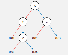
In some cases, it may be more memory efficient to represent a continuous joint distribution as a decision tree in a manner similar to what we discussed for discrete joint distributions. The internal nodes compare variables against thresholds and the leaf nodes are density values. Figure $2.7$ shows a decision tree that represents the density function in figure 2.6.
Another useful distribution is the multivariate Gaussian distribution with the density function
$$
\mathcal{N}(\mathbf{x} \mid \mu, \Sigma)=\frac{1}{(2 \pi)^{n / 2}|\Sigma|^{1 / 2}} \exp \left(-\frac{1}{2}(\mathbf{x}-\boldsymbol{\mu})^{\top} \boldsymbol{\Sigma}^{-1}(\mathbf{x}-\boldsymbol{\mu})\right)
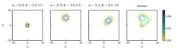
$$ where $\mathbf{x}$ is in $\mathbb{R}^{n}, \boldsymbol{\mu}$ is the mean vector, and $\boldsymbol{\Sigma}$ is the coovariance matrix. The density function above requires that $\Sigma$ be positive definite ${ }^{i \omega}$. The number of independent parameters is equal to $n+(n+1) n / 2$, the number of components in $\mu$ added to the number of components in the upper triangle of matrix $\Sigma^{11}$ Appendix B shows plots of different multivariate Gaussian density functions. We can also define multivariate Gaussian mixture models. Figure $2.8$ shows an example of one with three components.
统计代写
统计代写 | Statistical Learning and Decision Making代考|Joint Distributions
联合分布是多个变量的概率分布。单个变量上的分布称为单变量分布,多个变量上的分布称为多变量分布。如果我们有两个离散变量的联合分布X和是, 然后磷(X,是)表示两者的概率X=X和是=是.
从联合分布中,我们可以通过使用所谓的总概率定律对所有其他变量求和来计算一个变量或一组变量的边际分布:?
磷(X)=∑是磷(X,是)
本书通篇使用该属性。
现实世界的决策通常需要对涉及许多变量的联合分布进行推理。有时,重要的变量之间存在复杂的关系。我们可以使用不同的策略来表示联合分布,具体取决于变量是否涉及离散值或连续值。
统计代写 | Statistical Learning and Decision Making代考|Discrete Joint Distributions
如果变量是离散的,则联合分布可以用表 2.1 所示的表来表示。该表列出了三个二进制变量的所有可能赋值。每个变量只能是 0 或 1 ,导致23=8可能的任务。与其他离散分布一样,表中的概率总和必须为 1 。由此可见,虽然表中有八个条目,但其中只有七个是独立的。如果θ一世表示概率在一世表中的第 th 行,那么我们只需要参数θ1,…,θ7表示分布,因为我们知道θ8=1−(θ1+…+θ7).
如果我们有n二进制变量,那么我们需要尽可能多的2n−1指定联合分布的独立参数。参数数量的这种指数增长使得将分布存储在内存中变得困难。在某些情况下,我们可以假设我们的变量是独立的,这意味着一个的实现不会影响另一个的概率分布。如果X和是是独立的,有时写成X⊥是,那么我们知道磷(X,是)=磷(X)磷(是)
对全部X和是. 假设我们有二进制变量X1,…,Xn它们都是相互独立的,导致磷(X1:n)=∏一世磷(X一世). 这种分解允许我们仅用n独立参数而不是2n−1当我们不能假设独立时需要(见表2.2)。独立性可以在表示复杂性方面带来巨大的节省,但这通常是一个糟糕的假设。
我们可以用因子来表示联合分布。一个因素φ在一组变量上是从这些变量分配给实数的函数。为了表示概率分布,因子中的实数必须为非负数。可以对具有非负值的因子进行归一化,使其表示概率分布。算法 2.1 提供了离散因子的实现,以及示例2.3演示它们是如何工作的。
统计代写 | Statistical Learning and Decision Making代考|Continuous Joint Distributions
我们还可以定义连续变量的联合分布。一个相当简单的分布是多元均匀分布,它在任何有支持的地方分配一个恒定的概率密度。我们可以用在(一种,b)表示一个盒子上的均匀分布,它是区间的笛卡尔积一世间隔是[一种一世,b一世]. 这一系列均匀分布是一种特殊类型的多元乘积分布,它是根据单变量分布的乘积定义的分布。在这种情况下,
在(X∣一种,b)=∏一世在(X一世∣一种一世,b一世)
我们可以从多元均匀分布的加权集合创建混合模型,就像我们可以使用单变量分布一样。如果我们有一个联合分布n变量和ķ混合成分,我们需要定义ķ(2n+1)−1独立参数。对于每一个ķ除了权重之外,我们还需要为每个变量定义上限和下限。我们可以减去 1 因为权重总和必须为 1 。数字2.6显示了一个可以由五个组件表示的示例。
通过独立离散每个变量来表示分段常数密度函数也很常见。离散化由每个变量的一组 bin 边缘表示。这些 bin 边缘在变量上定义了一个网格。然后,我们将恒定概率密度与每个网格单元相关联。箱边缘不必均匀分离。在某些情况下,可能需要在某些值附近增加分辨率。不同的变量可能具有与之关联的不同 bin 边缘。如果有n变量和米每个变量的箱,那么我们需要米n−1除了定义 bin 边缘的值之外,定义分布的独立参数。
在某些情况下,以类似于我们讨论的离散联合分布的方式将连续联合分布表示为决策树可能更节省内存。内部节点将变量与阈值进行比较,叶节点是密度值。数字2.7显示了表示图 2.6 中的密度函数的决策树。
另一个有用的分布是具有密度函数的多元高斯分布
ñ(X∣μ,Σ)=1(2圆周率)n/2|Σ|1/2经验(−12(X−μ)⊤Σ−1(X−μ))在哪里X在Rn,μ是平均向量,并且Σ是协方差矩阵。上面的密度函数要求Σ是肯定的一世ω. 独立参数的数量等于n+(n+1)n/2, 中的组件数μ添加到矩阵的上三角形中的组件数Σ11附录 B 显示了不同的多元高斯密度函数图。我们还可以定义多元高斯混合模型。数字2.8显示了一个具有三个组件的示例。

统计代写请认准statistics-lab™. statistics-lab™为您的留学生涯保驾护航。
金融工程代写
金融工程是使用数学技术来解决金融问题。金融工程使用计算机科学、统计学、经济学和应用数学领域的工具和知识来解决当前的金融问题,以及设计新的和创新的金融产品。
非参数统计代写
非参数统计指的是一种统计方法,其中不假设数据来自于由少数参数决定的规定模型;这种模型的例子包括正态分布模型和线性回归模型。
广义线性模型代考
广义线性模型(GLM)归属统计学领域,是一种应用灵活的线性回归模型。该模型允许因变量的偏差分布有除了正态分布之外的其它分布。
术语 广义线性模型(GLM)通常是指给定连续和/或分类预测因素的连续响应变量的常规线性回归模型。它包括多元线性回归,以及方差分析和方差分析(仅含固定效应)。
有限元方法代写
有限元方法(FEM)是一种流行的方法,用于数值解决工程和数学建模中出现的微分方程。典型的问题领域包括结构分析、传热、流体流动、质量运输和电磁势等传统领域。
有限元是一种通用的数值方法,用于解决两个或三个空间变量的偏微分方程(即一些边界值问题)。为了解决一个问题,有限元将一个大系统细分为更小、更简单的部分,称为有限元。这是通过在空间维度上的特定空间离散化来实现的,它是通过构建对象的网格来实现的:用于求解的数值域,它有有限数量的点。边界值问题的有限元方法表述最终导致一个代数方程组。该方法在域上对未知函数进行逼近。[1] 然后将模拟这些有限元的简单方程组合成一个更大的方程系统,以模拟整个问题。然后,有限元通过变化微积分使相关的误差函数最小化来逼近一个解决方案。
tatistics-lab作为专业的留学生服务机构,多年来已为美国、英国、加拿大、澳洲等留学热门地的学生提供专业的学术服务,包括但不限于Essay代写,Assignment代写,Dissertation代写,Report代写,小组作业代写,Proposal代写,Paper代写,Presentation代写,计算机作业代写,论文修改和润色,网课代做,exam代考等等。写作范围涵盖高中,本科,研究生等海外留学全阶段,辐射金融,经济学,会计学,审计学,管理学等全球99%专业科目。写作团队既有专业英语母语作者,也有海外名校硕博留学生,每位写作老师都拥有过硬的语言能力,专业的学科背景和学术写作经验。我们承诺100%原创,100%专业,100%准时,100%满意。
随机分析代写
随机微积分是数学的一个分支,对随机过程进行操作。它允许为随机过程的积分定义一个关于随机过程的一致的积分理论。这个领域是由日本数学家伊藤清在第二次世界大战期间创建并开始的。
时间序列分析代写
随机过程,是依赖于参数的一组随机变量的全体,参数通常是时间。 随机变量是随机现象的数量表现,其时间序列是一组按照时间发生先后顺序进行排列的数据点序列。通常一组时间序列的时间间隔为一恒定值(如1秒,5分钟,12小时,7天,1年),因此时间序列可以作为离散时间数据进行分析处理。研究时间序列数据的意义在于现实中,往往需要研究某个事物其随时间发展变化的规律。这就需要通过研究该事物过去发展的历史记录,以得到其自身发展的规律。
回归分析代写
多元回归分析渐进(Multiple Regression Analysis Asymptotics)属于计量经济学领域,主要是一种数学上的统计分析方法,可以分析复杂情况下各影响因素的数学关系,在自然科学、社会和经济学等多个领域内应用广泛。
MATLAB代写
MATLAB 是一种用于技术计算的高性能语言。它将计算、可视化和编程集成在一个易于使用的环境中,其中问题和解决方案以熟悉的数学符号表示。典型用途包括:数学和计算算法开发建模、仿真和原型制作数据分析、探索和可视化科学和工程图形应用程序开发,包括图形用户界面构建MATLAB 是一个交互式系统,其基本数据元素是一个不需要维度的数组。这使您可以解决许多技术计算问题,尤其是那些具有矩阵和向量公式的问题,而只需用 C 或 Fortran 等标量非交互式语言编写程序所需的时间的一小部分。MATLAB 名称代表矩阵实验室。MATLAB 最初的编写目的是提供对由 LINPACK 和 EISPACK 项目开发的矩阵软件的轻松访问,这两个项目共同代表了矩阵计算软件的最新技术。MATLAB 经过多年的发展,得到了许多用户的投入。在大学环境中,它是数学、工程和科学入门和高级课程的标准教学工具。在工业领域,MATLAB 是高效研究、开发和分析的首选工具。MATLAB 具有一系列称为工具箱的特定于应用程序的解决方案。对于大多数 MATLAB 用户来说非常重要,工具箱允许您学习和应用专业技术。工具箱是 MATLAB 函数(M 文件)的综合集合,可扩展 MATLAB 环境以解决特定类别的问题。可用工具箱的领域包括信号处理、控制系统、神经网络、模糊逻辑、小波、仿真等。