如果你也在 怎样代写AP统计这个学科遇到相关的难题,请随时右上角联系我们的24/7代写客服。
AP统计学与大学的统计学课程在核心内容上是一致的,只是涉及的深度稍浅,AP统计学主要包含以下四部分内容。 第一部分 如何获取数据,获取数据的方式有哪些呢? 获取数据的方式主要包括普查、抽样调查、观测研究和实验设计等。
statistics-lab™ 为您的留学生涯保驾护航 在代写AP统计方面已经树立了自己的口碑, 保证靠谱, 高质且原创的统计Statistics代写服务。我们的专家在代写AP统计代写方面经验极为丰富,各种代写AP统计相关的作业也就用不着说。
我们提供的AP统计及其相关学科的代写,服务范围广, 其中包括但不限于:
- Statistical Inference 统计推断
- Statistical Computing 统计计算
- Advanced Probability Theory 高等概率论
- Advanced Mathematical Statistics 高等数理统计学
- (Generalized) Linear Models 广义线性模型
- Statistical Machine Learning 统计机器学习
- Longitudinal Data Analysis 纵向数据分析
- Foundations of Data Science 数据科学基础
统计代写|AP统计辅导AP统计答疑|The t-Distributions
- The Central Limit Theorem (CLT) is a very powerful tool, as was evident in the previous chapter. Our penny activity demonstrated that as long as we have a large enough sample, the sampling distribution of $\bar{x}$ is approximately normal. This is true no matter what the population distribution looks like. To use a z-statistic, however, we have to know the population standard deviation, $\sigma$. In the real world, $\sigma$ is usually unknown. Remember, we use statistical inference to make predictions about what we believe to be true about a population.
- When $\sigma$ is unknown, we estimate $\sigma$ with $s$. Recall that $s$ is the sample standard deviation. When using $s$ to estimate $\sigma$, the standard deviation of the sampling distribution for means is $s_{-}=\frac{s}{\sqrt{n}}$. When you use $s$ to estimate $\sigma$, the standard deviation of the sampling distribution is called the standard error of the sample mean, $\bar{x}$.
- While working for Guinness Brewing in Dublin, Ireland, William S. Gosset discovered that when he used $s$ to estimate $\sigma$, the shape of the sampling distribution changed depending on the sample size. This new distribution was not exactly normal. Gosset called this new distribution the $t$-distribution. It is sometimes referred to as the student’s $\mathbf{t}$.
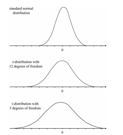
- The t-distribution, like the standard normal distribution, is singlepeaked, symmetrical, and bell shaped. It’s important to notice, as mentioned earlier, that as the sample size $(n)$ increases, the variability of the sampling distribution decreases. Thus, as the sample size increases, the t-distributions approach the standard normal model. When the sample size is small, there is more variability in the sampling distribution, and therefore there is more area (probability) under the density curve in the “tails” of the distribution. Since the area in the “tails” of the distribution is greater, the t-distributions are “flatter” than the standard normal curve. We refer to a t-distribution by its degrees of freedom. There are $n-1$ degrees of freedom. The ” $n-1$ ” degrees of freedom are used since we are using $s$ to estimate $\sigma$ and $s$ has $n-1$ degrees of freedom. Figure $7.1$ shows two different t-distributions with 3 and 12 degrees of freedom, respectively, along with the standard normal curve. It’s important to note that when dealing with a normal distribution, $z=\frac{\overline{x-\mu}}{\sigma / \sqrt{n}}$ and when working with a t-distribution, $t=\frac{\bar{x}-\mu}{s / \sqrt{n}}$. Using $s$ to estimate $\sigma$ introduces another source of variability into the statistic.
统计代写|AP统计辅导AP统计答疑|One-Sample t-Interval for the Mean
- As mentioned earlier, we use statistical inference when we wish to estimate some parameter of the population. Often, we want to estimate the mean of a population. Since we know that sample statistics usually vary, we will construct a confidence interval. The confidence interval will give a range of values that would be reasonable values for the parameter of interest, based on the statistic obtained from the sample.In this section, we will focus on creating a confidence interval for the mean of a population.
- When dealing with inference, we must always check certain assumptions for inference. This is imperative! These “assumptions” must be met for our inference to be reliable. We confirm or disconfirm these “assumptions” by checking the appropriate conditions. Throughout the remainder of this book, we will perform inference for different parameters of populations. We must always check that the assumptions are met before we draw conclusions about our population of interest. If the assumptions cannot be verified, our results may be inaccurate. For each type of inference, we will discuss the necessary assumptions and conditions.
- The assumptions and conditions for a one-sample t-interval or onesample t-test are as follows:The t-procedures (t-interval and t-test) are robust, meaning that the results of our t-interval or t-test would not change very much even though the assumptions of the procedure are violated.
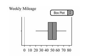
- Let’s discuss the assumptions and conditions. The first assumption is that the individuals or observations are independent. This should be true if our sample data is an SRS or if our data comes from a randomized experiment and if the sample size is less than $10 \%$ of the population size. The second assumption is that the population is normal. We may know or be given that the population is normal. If this is the case, we state this in our problem. If we do not know or if we are not told that the population is normal and the sample size is small, we must then look at a graph of the sample data. A histogram or a modified boxplot is probably best suited for looking at the sample data. If the sample size is less than 30 , we must be cautious of outliers or skewness in the data. Since normal distributions drop off quickly, it is unlikely to take a sample from a normal population and have the sample contain outliers or skewness. Outliers and strong skewness in a sample can be an indication that the population from which the sample is drawn might be non-normal. If the sample is large, we know that no matter what the population distribution looks like, we are guaranteed that the sampling distribution will be approximately normal. If you are asked to work on a problem for which the assumptions cannot be verified, state that this is the case and that the results of the inference being performed may be inaccurate.
统计代写|AP统计辅导AP统计答疑|Interpreting Confidence Intervals
It is highly likely that your understanding of how to interpret a confidence interval will be tested on the AP* Exam. What exactly can we say when we interpret the confidence interval in the context of the problem? In Example 1, we concluded, with $90 \%$ confidence, that $\mu$ was between $44.314$ and $54.286$ miles. That is, the average number of miles run by a typical male high-school cross-country runner in the state of Indiana is between $44.314$ and $54.286$. What exactly does this mean? Here’s what we can say: We can say that if this process were repeated many times, approximately $90 \%$ of all confidence intervals that we construct would contain the true mean. That is, if we were to obtain 100 different samples, find the mean of each sample, and construct 100 different confidence intervals, we would expect about 90 of them to contain the true population mean, $\mu$. That is also to say that about 10 of our confidence intervals would not contain the true population mean. No matter how carefully we obtain our random sample, there will always be sampling variability, and this variability makes the process imperfect. Be Careful! We cannot say that there is a $90 \%$ probability that the true mean is between $44.314$ and $54.286$ miles. We cannot say that $90 \%$ of all males cross-country runners in the state of Indiana run between $44.314$ and $54.286$ miles per week on average. These and comments like these are common on multiplechoice questions on exams. We can only say that if this process were repeated many times, $90 \%$ of all confidence intervals that we construct would contain the true population mean (Figure 7.3).
AP统计代写
统计代写|AP统计辅导AP统计答疑|The t-Distributions
- 中心极限定理 (CLT) 是一个非常强大的工具,如前一章所述。我们的一分钱活动表明,只要我们有足够大的样本,样本分布X¯大约是正常的。无论人口分布如何,这都是正确的。然而,要使用 z 统计量,我们必须知道总体标准差,σ. 在现实世界,σ通常是未知的。请记住,我们使用统计推断来预测我们认为关于人口的真实情况。
- 什么时候σ未知,我们估计σ和s. 回想起那个s是样本标准差。使用时s估计σ,均值的抽样分布的标准差为s−=sn. 当你使用s估计σ,抽样分布的标准差称为样本均值的标准差,X¯.
- 在爱尔兰都柏林为 Guinness Brewing 工作时,William S. Gosset 发现,当他使用s估计σ,采样分布的形状根据样本大小而变化。这种新的分布并不完全正常。Gosset 将这种新发行版称为吨-分配。它有时被称为学生的吨.
- t 分布与标准正态分布一样,是单峰的、对称的和钟形的。如前所述,重要的是要注意,作为样本量(n)增加,抽样分布的可变性减小。因此,随着样本量的增加,t 分布接近标准正态模型。当样本量较小时,抽样分布的变异性较大,因此分布“尾部”的密度曲线下面积(概率)较大。由于分布“尾部”的面积更大,因此 t 分布比标准正态曲线“更平坦”。我们通过其自由度来指代 t 分布。有n−1自由程度。这 ”n−1” 使用自由度,因为我们正在使用s估计σ和s拥有n−1自由程度。数字7.1显示了两个不同的 t 分布,分别具有 3 和 12 个自由度,以及标准正态曲线。需要注意的是,在处理正态分布时,和=X−μ¯σ/n在使用 t 分布时,吨=X¯−μs/n. 使用s估计σ在统计中引入了另一个可变性来源。
统计代写|AP统计辅导AP统计答疑|One-Sample t-Interval for the Mean
- 如前所述,当我们希望估计总体的某些参数时,我们会使用统计推断。通常,我们想要估计总体的平均值。由于我们知道样本统计数据通常会有所不同,因此我们将构建一个置信区间。根据从样本中获得的统计数据,置信区间将给出一系列值,这些值对于感兴趣的参数来说是合理的值。在本节中,我们将重点关注为总体平均值创建置信区间。
- 在处理推理时,我们必须始终检查某些假设以进行推理。这是必须的!必须满足这些“假设”才能使我们的推论可靠。我们通过检查适当的条件来确认或不确认这些“假设”。在本书的其余部分,我们将对不同的总体参数进行推断。在我们得出关于我们感兴趣的人群的结论之前,我们必须始终检查这些假设是否得到满足。如果假设无法验证,我们的结果可能不准确。对于每种类型的推理,我们将讨论必要的假设和条件。
- 单样本 t 区间或单样本 t 检验的假设和条件如下: t 过程(t 区间和 t 检验)是稳健的,这意味着我们的 t 区间或 t 检验的结果即使违反了程序的假设,也不会发生太大变化。
- 让我们讨论假设和条件。第一个假设是个体或观察是独立的。如果我们的样本数据是 SRS,或者我们的数据来自随机实验并且样本量小于10%的人口规模。第二个假设是人口是正常的。我们可能知道或被给予人口是正常的。如果是这种情况,我们会在问题中说明这一点。如果我们不知道或没有被告知总体正常且样本量很小,那么我们必须查看样本数据的图表。直方图或修改后的箱线图可能最适合查看样本数据。如果样本量小于 30 ,我们必须小心数据中的异常值或偏度。由于正态分布迅速下降,因此不太可能从正态总体中抽取样本并使样本包含异常值或偏度。样本中的异常值和强烈偏度可能表明从中抽取样本的总体可能是非正态的。如果样本很大,我们知道,无论总体分布如何,我们都可以保证抽样分布是近似正态的。如果您被要求处理无法验证假设的问题,请说明情况确实如此,并且执行的推理结果可能不准确。
统计代写|AP统计辅导AP统计答疑|Interpreting Confidence Intervals
您对如何解释置信区间的理解很可能会在 AP* 考试中得到检验。当我们在问题的背景下解释置信区间时,我们究竟能说什么?在示例 1 中,我们得出结论,90%信心,那μ介于44.314和54.286英里。也就是说,印第安纳州一个典型的男性高中越野跑者跑的平均英里数在44.314和54.286. 这到底是什么意思?这是我们可以说的:我们可以说,如果这个过程被重复很多次,大约90%在我们构建的所有置信区间中,都将包含真实均值。也就是说,如果我们要获得 100 个不同的样本,找到每个样本的均值,并构建 100 个不同的置信区间,我们预计其中大约 90 个包含真实的总体均值,μ. 也就是说,我们大约有 10 个置信区间不包含真实的总体均值。无论我们多么仔细地获得我们的随机样本,总会有抽样的可变性,而这种可变性使这个过程变得不完美。当心!我们不能说有一个90%真实均值在之间的概率44.314和54.286英里。我们不能这么说90%在印第安纳州的所有男性越野跑者中,44.314和54.286平均每周英里。这些和类似的评论在考试的多项选择题中很常见。我们只能说,如果这个过程重复多次,90%我们构建的所有置信区间将包含真实的总体均值(图 7.3)。

统计代写请认准statistics-lab™. statistics-lab™为您的留学生涯保驾护航。
金融工程代写
金融工程是使用数学技术来解决金融问题。金融工程使用计算机科学、统计学、经济学和应用数学领域的工具和知识来解决当前的金融问题,以及设计新的和创新的金融产品。
非参数统计代写
非参数统计指的是一种统计方法,其中不假设数据来自于由少数参数决定的规定模型;这种模型的例子包括正态分布模型和线性回归模型。
广义线性模型代考
广义线性模型(GLM)归属统计学领域,是一种应用灵活的线性回归模型。该模型允许因变量的偏差分布有除了正态分布之外的其它分布。
术语 广义线性模型(GLM)通常是指给定连续和/或分类预测因素的连续响应变量的常规线性回归模型。它包括多元线性回归,以及方差分析和方差分析(仅含固定效应)。
有限元方法代写
有限元方法(FEM)是一种流行的方法,用于数值解决工程和数学建模中出现的微分方程。典型的问题领域包括结构分析、传热、流体流动、质量运输和电磁势等传统领域。
有限元是一种通用的数值方法,用于解决两个或三个空间变量的偏微分方程(即一些边界值问题)。为了解决一个问题,有限元将一个大系统细分为更小、更简单的部分,称为有限元。这是通过在空间维度上的特定空间离散化来实现的,它是通过构建对象的网格来实现的:用于求解的数值域,它有有限数量的点。边界值问题的有限元方法表述最终导致一个代数方程组。该方法在域上对未知函数进行逼近。[1] 然后将模拟这些有限元的简单方程组合成一个更大的方程系统,以模拟整个问题。然后,有限元通过变化微积分使相关的误差函数最小化来逼近一个解决方案。
tatistics-lab作为专业的留学生服务机构,多年来已为美国、英国、加拿大、澳洲等留学热门地的学生提供专业的学术服务,包括但不限于Essay代写,Assignment代写,Dissertation代写,Report代写,小组作业代写,Proposal代写,Paper代写,Presentation代写,计算机作业代写,论文修改和润色,网课代做,exam代考等等。写作范围涵盖高中,本科,研究生等海外留学全阶段,辐射金融,经济学,会计学,审计学,管理学等全球99%专业科目。写作团队既有专业英语母语作者,也有海外名校硕博留学生,每位写作老师都拥有过硬的语言能力,专业的学科背景和学术写作经验。我们承诺100%原创,100%专业,100%准时,100%满意。
随机分析代写
随机微积分是数学的一个分支,对随机过程进行操作。它允许为随机过程的积分定义一个关于随机过程的一致的积分理论。这个领域是由日本数学家伊藤清在第二次世界大战期间创建并开始的。
时间序列分析代写
随机过程,是依赖于参数的一组随机变量的全体,参数通常是时间。 随机变量是随机现象的数量表现,其时间序列是一组按照时间发生先后顺序进行排列的数据点序列。通常一组时间序列的时间间隔为一恒定值(如1秒,5分钟,12小时,7天,1年),因此时间序列可以作为离散时间数据进行分析处理。研究时间序列数据的意义在于现实中,往往需要研究某个事物其随时间发展变化的规律。这就需要通过研究该事物过去发展的历史记录,以得到其自身发展的规律。
回归分析代写
多元回归分析渐进(Multiple Regression Analysis Asymptotics)属于计量经济学领域,主要是一种数学上的统计分析方法,可以分析复杂情况下各影响因素的数学关系,在自然科学、社会和经济学等多个领域内应用广泛。
MATLAB代写
MATLAB 是一种用于技术计算的高性能语言。它将计算、可视化和编程集成在一个易于使用的环境中,其中问题和解决方案以熟悉的数学符号表示。典型用途包括:数学和计算算法开发建模、仿真和原型制作数据分析、探索和可视化科学和工程图形应用程序开发,包括图形用户界面构建MATLAB 是一个交互式系统,其基本数据元素是一个不需要维度的数组。这使您可以解决许多技术计算问题,尤其是那些具有矩阵和向量公式的问题,而只需用 C 或 Fortran 等标量非交互式语言编写程序所需的时间的一小部分。MATLAB 名称代表矩阵实验室。MATLAB 最初的编写目的是提供对由 LINPACK 和 EISPACK 项目开发的矩阵软件的轻松访问,这两个项目共同代表了矩阵计算软件的最新技术。MATLAB 经过多年的发展,得到了许多用户的投入。在大学环境中,它是数学、工程和科学入门和高级课程的标准教学工具。在工业领域,MATLAB 是高效研究、开发和分析的首选工具。MATLAB 具有一系列称为工具箱的特定于应用程序的解决方案。对于大多数 MATLAB 用户来说非常重要,工具箱允许您学习和应用专业技术。工具箱是 MATLAB 函数(M 文件)的综合集合,可扩展 MATLAB 环境以解决特定类别的问题。可用工具箱的领域包括信号处理、控制系统、神经网络、模糊逻辑、小波、仿真等。