如果你也在 怎样代写利率建模Interest Rate Modeling这个学科遇到相关的难题,请随时右上角联系我们的24/7代写客服。
利率模型是指一种对利率的运动和演变进行建模的数学方法。它是一种基于市场风险的单因素短利率模型。瓦西克利率模型常用于经济学中,以确定利率在未来的移动方向。
statistics-lab™ 为您的留学生涯保驾护航 在代写利率建模Interest Rate Modeling方面已经树立了自己的口碑, 保证靠谱, 高质且原创的统计Statistics代写服务。我们的专家在代写利率建模Interest Rate Modeling代写方面经验极为丰富,各种代写利率建模Interest Rate Modeling相关的作业也就用不着说。
我们提供的利率建模Interest Rate Modeling及其相关学科的代写,服务范围广, 其中包括但不限于:
- Statistical Inference 统计推断
- Statistical Computing 统计计算
- Advanced Probability Theory 高等概率论
- Advanced Mathematical Statistics 高等数理统计学
- (Generalized) Linear Models 广义线性模型
- Statistical Machine Learning 统计机器学习
- Longitudinal Data Analysis 纵向数据分析
- Foundations of Data Science 数据科学基础
金融代写|利率建模代写Interest Rate Modeling代考|LIBOR Market Model
The LIBOR market model was introduced by Miltersen et al. (1997), Brace et al. (1997; hereinafter, BGM), Musiela and Rutkowski (1997), and Jamshidian $(1997)$. The notable points of this model are listed here:
- The model has positive LIBOR.
- The model admits an arbitrary deterministic volatility structure.
- The price formulae of a caplet and a floorlet are derived so as to be consistent with the corresponding Black’s price.
- An approximated price formula for a swaption is derived.
From these, the LIBOR market model has a usability advantage in calibration, and so it is widely applied as a standard model for derivatives pricing. As a particular example, the BGM model is the most well-known type of LIBOR market model, and is built in the HJM framework. The BGM approach requires a kind of differentiability for LIBOR volatility. It is impossible to satisfy this smoothness in practice because the volatility cannot be constructed except as a piecewise continuous, but not necessarily smooth, function. Because of this, the BGM model is not strictly supported in the HJM framework. For more advanced study of this problem, see Yasuoka (2001, 2013b).
At one end of the spectrum of models, the approaches by Musiela and Rutkowski (1997) and Jamshidian (1997) stand on a martingale pricing theory, with no theoretical imperfections. However, their models are constructed under a risk-neutral measure without referring to the real-world measure.
In this section and the next, we introduce the LIBOR market model as described by Jamshidian (1997). Because the topic of this book is risk management, pricing of derivatives is not addressed here at length. For a more advanced treatment of pricing, readers are recommended to consult Brigo and Mercurio (2007) or Gatarek et al. (2007).
Similarly to the argument for the HJM model, when the LIBOR and bond prices are represented under a risk-neutral measure, we call the resulting system a risk-neutral model. When, instead, they are represented under $\mathbf{P}$, the resulting system is referred to as a real-world model. Strict definitions of these terms will be given later.
金融代写|利率建模代写Interest Rate Modeling代考|Existence of LIBOR Market Model
The existence of the LIBOR model is shown in the following theorem.
Theorem 5.2.1 For arbitrary deterministic volatility $\lambda_{i}(t), i=1, \cdots, n-1$, the LIBOR market model exists.
The LIBOR model can be constructed under any of several risk-neutral measures. Applying this, we will show the existence of the LIBOR model under the real-world measure in the next section, and show how the models are implied under other measures in Sections $5.4$ and $5.5$ of this chapter. It is thought that this approach is the simplest method of constructing the LIBOR market model for practical use. Therefore, we here only sketch Jamshidian’s LIBOR market model under a forward measure, omitting the proof.
Let each of $\lambda_{i}(t)$ be an arbitrary deterministic function in $t$ for $i=1, \cdots, n-$
- Consider the following equation:
$$
\frac{d L_{i}(t)}{L_{i}(t)}=\sum_{j=i+1}^{n-1} \frac{\delta_{j} L_{j}(t) \lambda_{i}(t) \lambda_{j}(t)}{1+\delta_{j} L_{j}} d t+\lambda_{i}(t) d Z_{t}
$$
Here, $Z_{t}$ is a $d$-dimensional Brownian motion with respect to a measure $\mathbf{Q}(\sim$ $\mathbf{P})$. With this setup, the following proposition is given in Jamshidian ( 1997 , Corollary 2.1).
Proposition 5.2.2 The equation (5.4) admits a unique positive solution for an arbitrary initial condition $L_{i}(0)>0$ for all i. Further, $Y_{i}(t)=(1+$ $\left.\delta_{i} L_{i}(t)\right) \cdots\left(1+\delta_{i} L_{n-1}(t)\right)$ is a $\mathbf{Q}$-martingale.
Let $B_{n}(t)$ be an arbitrary bond price process such that $B_{n}\left(T_{n}\right)=1$ and
$$
B_{n}\left(T_{i}\right)=\frac{1}{\prod_{j=i}^{n-1}\left(1+\delta_{j} L_{j}\left(T_{j}\right)\right)}
$$ at each $T_{i}$. Accordingly, we define $B_{i}(t)$ for $i<n$ by
$$
\frac{B_{i}(t)}{B_{n}(t)}=\prod_{j=i}^{n-1}\left(1+\delta_{j} L_{j}(t)\right)
$$
From these, we see that $B_{i}\left(T_{i}\right)=1$ and the relation (5.2) is satisfied for all $i$. By Proposition 5.2.2, $\prod_{j=i}^{n-1}\left(1+\delta_{j} L_{j}(t)\right)$ is a Q-martingale for every $i$. Hence $B_{i}(t) / B_{n}(t)$ is a Q-martingale for all $i$.
Along these lines, $\mathbf{Q}$ is a $B_{n}$ numéraire measure and is referred to as a forward measure. As a result, the bond market $\mathcal{B}$ is arbitrage-free from Theorem $3.2 .2$
金融代写|利率建模代写Interest Rate Modeling代考|LIBOR Market Model under a Real-world Measure
Within the same setting as in Sections $5.1$ and 5.2, we give a definition of the LMRW and show the existence of the model, following Yasuoka (2013a).
Definition 5.3 The bond market $\mathcal{B}$ is called the $L M R W$ when the following conditions are satisfied.
- The LIBOR processes $L_{i}, i=1, \cdots, n$, with $L_{i}(t)>0$, are represented under the real-world measure $\mathbf{P}$ such that each volatility $\lambda_{i}(t)$ and the market price of risk $\varphi_{t}$ are deterministic in $t$.
- The bond market $\mathcal{B}$ is arbitrage-free; here this means that $B_{i}(t) \in \mathcal{B}, i=$ $1, \cdots, n$ and the state price deflator $\xi_{t}$ are positive Ito processes represented under $\mathbf{P}$.
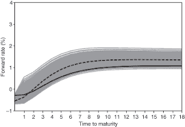
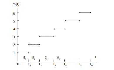
For this, we define a left-continuous function $m(t)$ by $m(t)=j$, while $t \in$ $\left(T_{j-1}, T_{j}\right]$. Succinctly, $m(t)$ represents the index of the next maturity date $.$ Examination of Fig. $5.1$ may help to see the features of $m(t)$.
To show the existence of the LMRW, it is sufficient to give the simplest example for arbitrarily given volatility $\lambda$ and market price of risk $\varphi$. For this, we define a process $\bar{\mu}(t)$ by $\bar{\mu}(t)=\bar{\mu}\left(T_{m(t)}\right)$ such that
$$
\bar{\mu}\left(T_{i}\right)=\frac{1}{\delta_{i-1}} \log \left{1+\delta_{i-1} L_{i-1}\left(T_{i-1}\right)\right}
$$
at each time $T_{i}$. Specifically, $\bar{\mu}(t)$ represents the yield for the shortest maturity bond, with the next maturity $T_{m(t)}$. As a consequence, $\bar{\mu}(t)$ is constant on each period $\left(T_{i-1}, T_{i}\right], i=1, \cdots, n$.
Let $\varphi_{t}$ be an arbitrarily given market price of risk such that $\varphi_{l}$ is an $\mathbf{R}^{d}-$ valued deterministic function with
$$
\int_{0}^{T}\left|\varphi_{t}\right|^{2} d s<\infty $$ Let $\lambda_{i}(t), i=1, \cdots, n$ be deterministic volatilities. We set $\chi_{i}(t)$ as $$ \chi_{i}(t)=\frac{\lambda_{i}(t) \delta_{i} L_{i}(t)}{1+\delta_{i} L_{i}(t)} ; i=1, \cdots, n . $$ Consider the following equation with the initial LIBOR $L_{i}(0)>0$,
$$
\frac{d L_{i}(t)}{L_{i}(t)}=\left{\lambda_{i}(t) \sum_{j=m(t)}^{i} \chi_{j}(t)+\lambda_{i}(t) \varphi_{t}\right} d t+\lambda_{i}(t) d W_{t}
$$
for $i=1, \cdots, n$. It is known that the solution $L_{i}(t)$ exists uniquely and $L_{i}(t)>$ 0 . We assume that bond price processes $B_{i}(t), i=1, \cdots, n$ are Ito processes with initial values $B_{0}(0)=1$ and
$$
B_{i}(0)=\prod_{j=0}^{i-1}\left(1+\delta_{j} L_{j}(0)\right)^{-1}
$$ such that
$$
\frac{d B_{i}(t)}{B_{i}(t)}=\left{\bar{\mu}(t)-\sum_{j=m(t)}^{i-1} \chi_{j}(t) \varphi_{t}\right} d t-\sum_{j=m(t)}^{i-1} \chi_{j}(t) d W_{t} .
$$
Under this setup, we give the following theorem, which shows the existence of the LMRW.
利率建模代考
金融代写|利率建模代写Interest Rate Modeling代考|LIBOR Market Model
LIBOR 市场模型由 Miltersen 等人引入。(1997 年),布雷斯等人。(1997 年;以下称为 BGM)、Musiela 和 Rutkowski(1997 年)和 Jamshidian(1997). 此处列出了此模型的值得注意的点:
- 该模型具有正 LIBOR。
- 该模型允许任意确定的波动率结构。
- 导出caplet和floorlet的价格公式以与对应的布莱克价格一致。
- 导出了互换期权的近似价格公式。
由此可见,LIBOR 市场模型在校准方面具有可用性优势,因此被广泛用作衍生品定价的标准模型。作为一个具体的例子,BGM 模型是最知名的 LIBOR 市场模型类型,并且构建在 HJM 框架中。BGM 方法需要一种 LIBOR 波动性的可微性。在实践中不可能满足这种平滑性,因为波动率只能构建为分段连续但不一定平滑的函数。因此,HJM 框架并不严格支持 BGM 模型。有关此问题的更高级研究,请参阅 Yasuoka (2001, 2013b)。
在模型范围的一端,Musiela 和 Rutkowski (1997) 和 Jamshidian (1997) 的方法基于鞅定价理论,没有理论缺陷。然而,他们的模型是在风险中性的衡量标准下构建的,没有参考现实世界的衡量标准。
在本节和下一节中,我们将介绍 Jamshidian (1997) 所描述的 LIBOR 市场模型。因为本书的主题是风险管理,衍生品的定价在这里没有详细讨论。对于更高级的定价处理,建议读者参考 Brigo 和 Mercurio (2007) 或 Gatarek 等人。(2007 年)。
与 HJM 模型的论点类似,当 LIBOR 和债券价格在风险中性度量下表示时,我们称所得系统为风险中性模型。相反,当它们被表示为磷,得到的系统被称为真实世界模型。这些术语的严格定义将在后面给出。
金融代写|利率建模代写Interest Rate Modeling代考|Existence of LIBOR Market Model
LIBOR 模型的存在如下定理所示。
定理 5.2.1 对于任意确定性波动率λ一世(吨),一世=1,⋯,n−1, LIBOR 市场模型存在。
LIBOR 模型可以在多种风险中性措施中的任何一种下构建。应用这一点,我们将在下一节中展示 LIBOR 模型在真实世界度量下的存在,并展示模型在其他度量下的隐含部分5.4和5.5本章的。这种方法被认为是构建 LIBOR 市场模型以供实际使用的最简单方法。因此,我们这里只勾勒出Jamshidian 的LIBOR 市场模型在前向测度下,省略了证明。
让每一个λ一世(吨)是任意确定性函数吨为了一世=1,⋯,n−
- 考虑以下等式:
d大号一世(吨)大号一世(吨)=∑j=一世+1n−1dj大号j(吨)λ一世(吨)λj(吨)1+dj大号jd吨+λ一世(吨)d从吨
这里,从吨是一个d关于测度的一维布朗运动问(∼ 磷). 通过这种设置,Jamshidian (1997, Corollary 2.1) 给出了以下命题。
命题 5.2.2 方程 (5.4) 承认任意初始条件的唯一正解大号一世(0)>0对于所有我。更远,是一世(吨)=(1+ d一世大号一世(吨))⋯(1+d一世大号n−1(吨))是一个问-鞅。
让乙n(吨)是一个任意的债券价格过程,使得乙n(吨n)=1和
乙n(吨一世)=1∏j=一世n−1(1+dj大号j(吨j))在每一个吨一世. 因此,我们定义乙一世(吨)为了一世<n经过
乙一世(吨)乙n(吨)=∏j=一世n−1(1+dj大号j(吨))
从这些我们可以看出乙一世(吨一世)=1并且关系(5.2)满足所有一世. 根据提案 5.2.2,∏j=一世n−1(1+dj大号j(吨))是每一个 Q-鞅一世. 因此乙一世(吨)/乙n(吨)是所有人的 Q-鞅一世.
沿着这些思路,问是一个乙nnuméraire measure,被称为远期测量。因此,债券市场乙从定理无套利3.2.2
金融代写|利率建模代写Interest Rate Modeling代考|LIBOR Market Model under a Real-world Measure
在与部分相同的设置中5.1和 5.2,我们给出了 LMRW 的定义,并表明模型的存在,遵循 Yasuoka (2013a)。
定义 5.3 债券市场乙被称为大号米R在当满足以下条件时。
- LIBOR 流程大号一世,一世=1,⋯,n, 和大号一世(吨)>0, 在真实世界的度量下表示磷这样每个波动率λ一世(吨)和风险的市场价格披吨是确定性的吨.
- 债券市场乙无套利;这意味着乙一世(吨)∈乙,一世= 1,⋯,n和国家价格平减指数X吨是正 Ito 过程表示下磷.
为此,我们定义了一个左连续函数米(吨)经过米(吨)=j, 尽管吨∈ (吨j−1,吨j]. 简而言之,米(吨)代表下一个到期日的指数.图的检查5.1可能有助于了解米(吨).
为了证明 LMRW 的存在,给出任意给定波动率的最简单的例子就足够了λ和市场风险价格披. 为此,我们定义了一个流程μ¯(吨)经过μ¯(吨)=μ¯(吨米(吨))这样
\bar{\mu}\left(T_{i}\right)=\frac{1}{\delta_{i-1}} \log \left{1+\delta_{i-1} L_{i-1 }\left(T_{i-1}\right)\right}\bar{\mu}\left(T_{i}\right)=\frac{1}{\delta_{i-1}} \log \left{1+\delta_{i-1} L_{i-1 }\left(T_{i-1}\right)\right}
每次吨一世. 具体来说,μ¯(吨)代表最短期限债券的收益率,下一个到期日吨米(吨). 作为结果,μ¯(吨)在每个时期都是恒定的(吨一世−1,吨一世],一世=1,⋯,n.
让披吨是任意给定的市场风险价格,使得披l是一个Rd−有值的确定性函数
∫0吨|披吨|2ds<∞让λ一世(吨),一世=1,⋯,n是确定性的波动率。我们设置χ一世(吨)作为
χ一世(吨)=λ一世(吨)d一世大号一世(吨)1+d一世大号一世(吨);一世=1,⋯,n.考虑以下具有初始 LIBOR 的等式大号一世(0)>0,
\frac{d L_{i}(t)}{L_{i}(t)}=\left{\lambda_{i}(t) \sum_{j=m(t)}^{i} \chi_{ j}(t)+\lambda_{i}(t) \varphi_{t}\right} d t+\lambda_{i}(t) d W_{t}\frac{d L_{i}(t)}{L_{i}(t)}=\left{\lambda_{i}(t) \sum_{j=m(t)}^{i} \chi_{ j}(t)+\lambda_{i}(t) \varphi_{t}\right} d t+\lambda_{i}(t) d W_{t}
为了一世=1,⋯,n. 据了解,解决方案大号一世(吨)唯一存在并且大号一世(吨)>0 . 我们假设债券价格过程乙一世(吨),一世=1,⋯,n是具有初始值的 Ito 过程乙0(0)=1和
乙一世(0)=∏j=0一世−1(1+dj大号j(0))−1这样
\frac{d B_{i}(t)}{B_{i}(t)}=\left{\bar{\mu}(t)-\sum_{j=m(t)}^{i-1 } \chi_{j}(t) \varphi_{t}\right} d t-\sum_{j=m(t)}^{i-1} \chi_{j}(t) d W_{t} 。\frac{d B_{i}(t)}{B_{i}(t)}=\left{\bar{\mu}(t)-\sum_{j=m(t)}^{i-1 } \chi_{j}(t) \varphi_{t}\right} d t-\sum_{j=m(t)}^{i-1} \chi_{j}(t) d W_{t} 。
在这种设置下,我们给出了以下定理,它表明了 LMRW 的存在。

统计代写请认准statistics-lab™. statistics-lab™为您的留学生涯保驾护航。
金融工程代写
金融工程是使用数学技术来解决金融问题。金融工程使用计算机科学、统计学、经济学和应用数学领域的工具和知识来解决当前的金融问题,以及设计新的和创新的金融产品。
非参数统计代写
非参数统计指的是一种统计方法,其中不假设数据来自于由少数参数决定的规定模型;这种模型的例子包括正态分布模型和线性回归模型。
广义线性模型代考
广义线性模型(GLM)归属统计学领域,是一种应用灵活的线性回归模型。该模型允许因变量的偏差分布有除了正态分布之外的其它分布。
术语 广义线性模型(GLM)通常是指给定连续和/或分类预测因素的连续响应变量的常规线性回归模型。它包括多元线性回归,以及方差分析和方差分析(仅含固定效应)。
有限元方法代写
有限元方法(FEM)是一种流行的方法,用于数值解决工程和数学建模中出现的微分方程。典型的问题领域包括结构分析、传热、流体流动、质量运输和电磁势等传统领域。
有限元是一种通用的数值方法,用于解决两个或三个空间变量的偏微分方程(即一些边界值问题)。为了解决一个问题,有限元将一个大系统细分为更小、更简单的部分,称为有限元。这是通过在空间维度上的特定空间离散化来实现的,它是通过构建对象的网格来实现的:用于求解的数值域,它有有限数量的点。边界值问题的有限元方法表述最终导致一个代数方程组。该方法在域上对未知函数进行逼近。[1] 然后将模拟这些有限元的简单方程组合成一个更大的方程系统,以模拟整个问题。然后,有限元通过变化微积分使相关的误差函数最小化来逼近一个解决方案。
tatistics-lab作为专业的留学生服务机构,多年来已为美国、英国、加拿大、澳洲等留学热门地的学生提供专业的学术服务,包括但不限于Essay代写,Assignment代写,Dissertation代写,Report代写,小组作业代写,Proposal代写,Paper代写,Presentation代写,计算机作业代写,论文修改和润色,网课代做,exam代考等等。写作范围涵盖高中,本科,研究生等海外留学全阶段,辐射金融,经济学,会计学,审计学,管理学等全球99%专业科目。写作团队既有专业英语母语作者,也有海外名校硕博留学生,每位写作老师都拥有过硬的语言能力,专业的学科背景和学术写作经验。我们承诺100%原创,100%专业,100%准时,100%满意。
随机分析代写
随机微积分是数学的一个分支,对随机过程进行操作。它允许为随机过程的积分定义一个关于随机过程的一致的积分理论。这个领域是由日本数学家伊藤清在第二次世界大战期间创建并开始的。
时间序列分析代写
随机过程,是依赖于参数的一组随机变量的全体,参数通常是时间。 随机变量是随机现象的数量表现,其时间序列是一组按照时间发生先后顺序进行排列的数据点序列。通常一组时间序列的时间间隔为一恒定值(如1秒,5分钟,12小时,7天,1年),因此时间序列可以作为离散时间数据进行分析处理。研究时间序列数据的意义在于现实中,往往需要研究某个事物其随时间发展变化的规律。这就需要通过研究该事物过去发展的历史记录,以得到其自身发展的规律。
回归分析代写
多元回归分析渐进(Multiple Regression Analysis Asymptotics)属于计量经济学领域,主要是一种数学上的统计分析方法,可以分析复杂情况下各影响因素的数学关系,在自然科学、社会和经济学等多个领域内应用广泛。
MATLAB代写
MATLAB 是一种用于技术计算的高性能语言。它将计算、可视化和编程集成在一个易于使用的环境中,其中问题和解决方案以熟悉的数学符号表示。典型用途包括:数学和计算算法开发建模、仿真和原型制作数据分析、探索和可视化科学和工程图形应用程序开发,包括图形用户界面构建MATLAB 是一个交互式系统,其基本数据元素是一个不需要维度的数组。这使您可以解决许多技术计算问题,尤其是那些具有矩阵和向量公式的问题,而只需用 C 或 Fortran 等标量非交互式语言编写程序所需的时间的一小部分。MATLAB 名称代表矩阵实验室。MATLAB 最初的编写目的是提供对由 LINPACK 和 EISPACK 项目开发的矩阵软件的轻松访问,这两个项目共同代表了矩阵计算软件的最新技术。MATLAB 经过多年的发展,得到了许多用户的投入。在大学环境中,它是数学、工程和科学入门和高级课程的标准教学工具。在工业领域,MATLAB 是高效研究、开发和分析的首选工具。MATLAB 具有一系列称为工具箱的特定于应用程序的解决方案。对于大多数 MATLAB 用户来说非常重要,工具箱允许您学习和应用专业技术。工具箱是 MATLAB 函数(M 文件)的综合集合,可扩展 MATLAB 环境以解决特定类别的问题。可用工具箱的领域包括信号处理、控制系统、神经网络、模糊逻辑、小波、仿真等。