如果你也在 怎样代写利率建模Interest Rate Modeling这个学科遇到相关的难题,请随时右上角联系我们的24/7代写客服。
利率模型是指一种对利率的运动和演变进行建模的数学方法。它是一种基于市场风险的单因素短利率模型。瓦西克利率模型常用于经济学中,以确定利率在未来的移动方向。
statistics-lab™ 为您的留学生涯保驾护航 在代写利率建模Interest Rate Modeling方面已经树立了自己的口碑, 保证靠谱, 高质且原创的统计Statistics代写服务。我们的专家在代写利率建模Interest Rate Modeling代写方面经验极为丰富,各种代写利率建模Interest Rate Modeling相关的作业也就用不着说。
我们提供的利率建模Interest Rate Modeling及其相关学科的代写,服务范围广, 其中包括但不限于:
- Statistical Inference 统计推断
- Statistical Computing 统计计算
- Advanced Probability Theory 高等概率论
- Advanced Mathematical Statistics 高等数理统计学
- (Generalized) Linear Models 广义线性模型
- Statistical Machine Learning 统计机器学习
- Longitudinal Data Analysis 纵向数据分析
- Foundations of Data Science 数据科学基础
金融代写|利率建模代写Interest Rate Modeling代考|The Hull–White Model
In the early days, many stochastic models were introduced to describe the dynamics of the short rate. As examples, see Cox et al. (1985; hereinafter,CIR), Ho and Lee (1986), Hull and White (1990), and Vasicek (1977), among others. A strong point of these models is their parsimoniousness. Additionally, these models are described by affine term structures. For details of affine models, readers are recommended to consult Duffie and Kan (1996), Björk $(2004)$, or Munk (2011).
It is known that the Ho-Lee model and the Hull-White model are special cases of the Gaussian HJM model. The Hull-White model, in particular, is one of the most popular models in many financial institutions. Following along these lines, this section introduces the Hull-White model as a special case of the HJM model.
Short rate process
Let us consider a one-dimensional process of the short rate $r(t)$ represented by
$$
d r(t)=\kappa\left{\theta(t)-r(t)+\frac{\sigma}{\kappa} \varphi_{t}\right} d t+\sigma d W_{t}
$$
where $W_{t}$ is a one-dimensional Brownian motion under the real-world measure $\mathbf{P} ; \kappa$ and $\sigma$ are positive constants; $\theta(t)$ is a positive process; and $\varphi_{t}$ denotes the market price of risk.
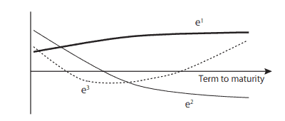
It is empirically observed that the volatility of long-term interest rates is less than that of short term rates, reflecting a general phenomenon referred to as mean reversion. To model this feature, the rate at which $r(t)$ reverts to $\theta(t)$ is the speed $\kappa$, called the mean reversion rate.
The savings account $B_{t}=\exp \left{\int_{0}^{t} r(s) d s\right}$ is taken as a numéraire. We set $Z_{t}=\int_{0}^{t} \varphi_{s} d s+W_{t}$. By the Girsanov theorem, there exists a risk-neutral measure $\mathbf{Q}$ equivalent to $\mathbf{P}$ such that $Z_{t}$ is a Brownian motion under $\mathbf{Q}$. From these, the short rate $r(t)$ is represented under $\mathbf{Q}$ as
$$
d r(t)=\kappa(\theta(t)-r(t)) d t+\sigma d Z_{t}
$$
It is known that the price of a zero-coupon bond with maturity $T$ is given by
$$
B(t, T)=\exp {-a(t, T)-b(T-t) r(t)}
$$
金融代写|利率建模代写Interest Rate Modeling代考|VaR Computed in the Real-world
This section studies the reason that the VaR should be computed using a real-world model. For this purpose, the valuation of the VaR depends on the choice of measure. We use the following simple example to illustrate this. For simplicity, we assume a null discount rate in the following argument (i.e. the forward price is equal to the present price).
Suppose a binary bond with expiry at time $T$ and with payoff $X$ at $T$ is given as follows.
$$
\left{\begin{array}{l}
\text { If } L>5 \% \text { at } T, \text { then } X=0 \
\text { If } L \leq 5 \% \text { at } T, \text { then } X=1.01,
\end{array}\right.
$$
where $L$ indicates the 6 -month LIBOR at $T$. Succinctly, the payoff is determined by the level of the 6 -month LIBOR at the expiry date.
The price of this security is computed by using some interest rate model under some risk-neutral measure $\mathbf{Q}$. For the model, we assume the probability distribution of $L$ as
$$
\left{\begin{array}{r}
\mathrm{Q}(L>5 \%)=0.09 \% \
\mathbf{Q}(L \leq 5 \%)=99.01 \%
\end{array}\right.
$$
With this distribution, the arbitrage price of this bond at $t=0$ is calculated by
$$
(1.01 \times 0.9901+0 \times 0.0009) \times 1=1.00
$$ because of the assumption of a null discount rate.
We buy this bond at price $1.00$. Let us valuate the $99 \% \mathrm{VaR}$ of this bond for holding period $T$. We can sell this for the price $1.01$ at time $T$ at a probability of more than $99 \%$. The $99 \% \mathrm{VaR}$ is valuated as the profit of $-0.01(=1.00-1.01)$ under Q.
Next, we assume that historical observation estimates for the 6-month LIBOR are
$$
\left{\begin{array}{l}
\mathbf{P}(L>5 \%)=2 \% \
\mathbf{P}(L \leq 5 \%)=98 \%
\end{array}\right.
$$
金融代写|利率建模代写Interest Rate Modeling代考|Estimation of the Market Price of Risk
In empirical analysis concerning the term structure of interest rates, we are observing historical data under the real-world measure. To give an example, when we use the Hull-White model, the dynamics of the short rate is described from equation $(4.41)$ as
$$
d r(t)=\kappa\left{\theta(t)-r(t)+\frac{\sigma}{\kappa} \varphi_{t}\right} d t+\sigma d W_{t}
$$
To calibrate this model such that this equation explains the historical dynamics of the short rate, we must estimate the parameters $\sigma$ and $\kappa$ and the market price of risk $\varphi_{t}$. In this way, we inevitably estimate $\varphi_{t}$ as part of fitting any interest rate model with the historical dynamics of the interest rates.
Along these lines, there are many studies on estimating the market price of risk in the field of economics. Some papers in this vein are Ahn and Gao (1999), Cheridito et al. (2007), Cochrane and Piazzesi (2010), De Jong (2000), and Duffee (2002). However, there are few papers that explicitly describe the method used in estimating the market price of risk in short rate models. It is even more difficult to find such papers that work with forward rate models.
In this section, we briefly describe three approaches to estimating the market price of risk in short rate models. For a more advanced treatment of this subject, we study theoretical methods for estimating the market price of risk in the forward rate model from Chapter $6 .$
利率建模代考
金融代写|利率建模代写Interest Rate Modeling代考|The Hull–White Model
早期,引入了许多随机模型来描述短期利率的动态。例如,参见 Cox 等人。(1985 年;以下简称 CIR)、Ho 和 Lee(1986 年)、Hull 和 White(1990 年)和 Vasicek(1977 年)等。这些模型的一个优点是它们的简约性。此外,这些模型由仿射术语结构描述。关于仿射模型的详细信息,建议读者参考 Duffie and Kan (1996), Björk(2004),或蒙克(2011 年)。
众所周知,Ho-Lee 模型和 Hull-White 模型是高斯 HJM 模型的特例。赫尔-怀特模型尤其是许多金融机构中最流行的模型之一。沿着这些思路,本节介绍 Hull-White 模型作为 HJM 模型的一个特例。
短利率过程
让我们考虑一个短利率的一维过程r(吨)代表为
d r(t)=\kappa\left{\theta(t)-r(t)+\frac{\sigma}{\kappa} \varphi_{t}\right} d t+\sigma d W_{t}d r(t)=\kappa\left{\theta(t)-r(t)+\frac{\sigma}{\kappa} \varphi_{t}\right} d t+\sigma d W_{t}
在哪里在吨是真实世界测量下的一维布朗运动磷;ķ和σ是正常数;θ(吨)是一个积极的过程;和披吨表示风险的市场价格。
根据经验观察,长期利率的波动性小于短期利率的波动性,反映了一种被称为均值回归的普遍现象。为了对该特征进行建模,速率r(吨)恢复到θ(吨)是速度ķ,称为平均回复率。
储蓄账户B_{t}=\exp \left{\int_{0}^{t} r(s) d s\right}B_{t}=\exp \left{\int_{0}^{t} r(s) d s\right}被视为一个numéraire。我们设置从吨=∫0吨披sds+在吨. 根据 Girsanov 定理,存在风险中性测度问相当于磷这样从吨是下的布朗运动问. 从这些来看,短期利率r(吨)表示在问作为
dr(吨)=ķ(θ(吨)−r(吨))d吨+σd从吨
众所周知,到期零息债券的价格吨是(谁)给的
乙(吨,吨)=经验−一个(吨,吨)−b(吨−吨)r(吨)
金融代写|利率建模代写Interest Rate Modeling代考|VaR Computed in the Real-world
本节研究应使用真实世界模型计算 VaR 的原因。为此,VaR 的估值取决于度量的选择。我们使用下面的简单示例来说明这一点。为简单起见,我们在以下论点中假设折现率为零(即远期价格等于当前价格)。
假设一个二元债券在某个时间到期吨并有回报X在吨给出如下。
$$
\左{
如果 大号>5% 在 吨, 然后 X=0 如果 大号≤5% 在 吨, 然后 X=1.01,\正确的。
$$
在哪里大号表示 6 个月 LIBOR 在吨. 简而言之,收益取决于到期日的 6 个月 LIBOR 水平。
该证券的价格是通过在某种风险中性措施下使用某种利率模型来计算的问. 对于模型,我们假设概率分布为大号作为
$$
\left{
问(大号>5%)=0.09% 问(大号≤5%)=99.01%\正确的。
在一世吨H吨H一世sd一世s吨r一世b在吨一世○n,吨H和一个rb一世吨r一个G和pr一世C和○F吨H一世sb○nd一个吨$吨=0$一世sC一个lC在l一个吨和db是
(1.01 \times 0.9901+0 \times 0.0009) \times 1=1.00
$$ 因为假设零贴现率。
我们以价格购买该债券1.00. 让我们评估一下99%在一个R本期债券持有期吨. 我们可以卖这个价格1.01有时吨概率大于99%. 这99%在一个R被评估为利润−0.01(=1.00−1.01)Q下。
接下来,我们假设 6 个月 LIBOR 的历史观测估计值为
$$
\left{
磷(大号>5%)=2% 磷(大号≤5%)=98%\正确的。
$$
金融代写|利率建模代写Interest Rate Modeling代考|Estimation of the Market Price of Risk
在利率期限结构的实证分析中,我们是在现实世界的衡量标准下观察历史数据。举个例子,当我们使用 Hull-White 模型时,短期利率的动力学由方程描述(4.41)作为
d r(t)=\kappa\left{\theta(t)-r(t)+\frac{\sigma}{\kappa} \varphi_{t}\right} d t+\sigma d W_{t}d r(t)=\kappa\left{\theta(t)-r(t)+\frac{\sigma}{\kappa} \varphi_{t}\right} d t+\sigma d W_{t}
为了校准这个模型,使这个方程能够解释短期利率的历史动态,我们必须估计参数σ和ķ和风险的市场价格披吨. 这样,我们不可避免地估计披吨作为拟合任何利率模型与利率历史动态的一部分。
沿着这些思路,在经济学领域有许多关于估计风险市场价格的研究。这方面的一些论文是 Ahn 和 Gao (1999),Cheridito 等人。(2007)、Cochrane 和 Piazzesi (2010)、De Jong (2000) 和 Duffee (2002)。然而,很少有论文明确描述在短期利率模型中估计风险市场价格所使用的方法。更难找到适用于远期利率模型的此类论文。
在本节中,我们将简要描述在短期利率模型中估计风险市场价格的三种方法。为了对该主题进行更深入的处理,我们研究了在第 1 章的远期利率模型中估计风险市场价格的理论方法。6.

统计代写请认准statistics-lab™. statistics-lab™为您的留学生涯保驾护航。
金融工程代写
金融工程是使用数学技术来解决金融问题。金融工程使用计算机科学、统计学、经济学和应用数学领域的工具和知识来解决当前的金融问题,以及设计新的和创新的金融产品。
非参数统计代写
非参数统计指的是一种统计方法,其中不假设数据来自于由少数参数决定的规定模型;这种模型的例子包括正态分布模型和线性回归模型。
广义线性模型代考
广义线性模型(GLM)归属统计学领域,是一种应用灵活的线性回归模型。该模型允许因变量的偏差分布有除了正态分布之外的其它分布。
术语 广义线性模型(GLM)通常是指给定连续和/或分类预测因素的连续响应变量的常规线性回归模型。它包括多元线性回归,以及方差分析和方差分析(仅含固定效应)。
有限元方法代写
有限元方法(FEM)是一种流行的方法,用于数值解决工程和数学建模中出现的微分方程。典型的问题领域包括结构分析、传热、流体流动、质量运输和电磁势等传统领域。
有限元是一种通用的数值方法,用于解决两个或三个空间变量的偏微分方程(即一些边界值问题)。为了解决一个问题,有限元将一个大系统细分为更小、更简单的部分,称为有限元。这是通过在空间维度上的特定空间离散化来实现的,它是通过构建对象的网格来实现的:用于求解的数值域,它有有限数量的点。边界值问题的有限元方法表述最终导致一个代数方程组。该方法在域上对未知函数进行逼近。[1] 然后将模拟这些有限元的简单方程组合成一个更大的方程系统,以模拟整个问题。然后,有限元通过变化微积分使相关的误差函数最小化来逼近一个解决方案。
tatistics-lab作为专业的留学生服务机构,多年来已为美国、英国、加拿大、澳洲等留学热门地的学生提供专业的学术服务,包括但不限于Essay代写,Assignment代写,Dissertation代写,Report代写,小组作业代写,Proposal代写,Paper代写,Presentation代写,计算机作业代写,论文修改和润色,网课代做,exam代考等等。写作范围涵盖高中,本科,研究生等海外留学全阶段,辐射金融,经济学,会计学,审计学,管理学等全球99%专业科目。写作团队既有专业英语母语作者,也有海外名校硕博留学生,每位写作老师都拥有过硬的语言能力,专业的学科背景和学术写作经验。我们承诺100%原创,100%专业,100%准时,100%满意。
随机分析代写
随机微积分是数学的一个分支,对随机过程进行操作。它允许为随机过程的积分定义一个关于随机过程的一致的积分理论。这个领域是由日本数学家伊藤清在第二次世界大战期间创建并开始的。
时间序列分析代写
随机过程,是依赖于参数的一组随机变量的全体,参数通常是时间。 随机变量是随机现象的数量表现,其时间序列是一组按照时间发生先后顺序进行排列的数据点序列。通常一组时间序列的时间间隔为一恒定值(如1秒,5分钟,12小时,7天,1年),因此时间序列可以作为离散时间数据进行分析处理。研究时间序列数据的意义在于现实中,往往需要研究某个事物其随时间发展变化的规律。这就需要通过研究该事物过去发展的历史记录,以得到其自身发展的规律。
回归分析代写
多元回归分析渐进(Multiple Regression Analysis Asymptotics)属于计量经济学领域,主要是一种数学上的统计分析方法,可以分析复杂情况下各影响因素的数学关系,在自然科学、社会和经济学等多个领域内应用广泛。
MATLAB代写
MATLAB 是一种用于技术计算的高性能语言。它将计算、可视化和编程集成在一个易于使用的环境中,其中问题和解决方案以熟悉的数学符号表示。典型用途包括:数学和计算算法开发建模、仿真和原型制作数据分析、探索和可视化科学和工程图形应用程序开发,包括图形用户界面构建MATLAB 是一个交互式系统,其基本数据元素是一个不需要维度的数组。这使您可以解决许多技术计算问题,尤其是那些具有矩阵和向量公式的问题,而只需用 C 或 Fortran 等标量非交互式语言编写程序所需的时间的一小部分。MATLAB 名称代表矩阵实验室。MATLAB 最初的编写目的是提供对由 LINPACK 和 EISPACK 项目开发的矩阵软件的轻松访问,这两个项目共同代表了矩阵计算软件的最新技术。MATLAB 经过多年的发展,得到了许多用户的投入。在大学环境中,它是数学、工程和科学入门和高级课程的标准教学工具。在工业领域,MATLAB 是高效研究、开发和分析的首选工具。MATLAB 具有一系列称为工具箱的特定于应用程序的解决方案。对于大多数 MATLAB 用户来说非常重要,工具箱允许您学习和应用专业技术。工具箱是 MATLAB 函数(M 文件)的综合集合,可扩展 MATLAB 环境以解决特定类别的问题。可用工具箱的领域包括信号处理、控制系统、神经网络、模糊逻辑、小波、仿真等。